Broadband Packet Switching Technologies

output port 10. This operation repeats in other switches along the path to the destination. Once the connection is terminated, the call processor deletes the associated entries of the routing tables along the path.

In the multicast case, a cell is replicated into multiple copies and each copy is routed to an output port. Since the VPIrVCI of each copy at the output port can be different, VPIrVCI replacement usually takes place at the output instead of the input. As a result, the routing table is usually split into two parts, one at the input and the other at the output. The former has two fields in the RIT: the old VPIrVCI and the N-bit routing information. The latter has three fields in the RIT: the input port number, the old VPIrVCI, and the new VPIrVCI. The combination of the input port number and the old VPIrVCI can uniquely identify the multicast connection and is used as an index to locate the new VPIrVCI at the output. Since multiple VPIrVCIs from different input ports can merge to the same output port and have the identical old VPIrVCI value, it thus has to use extra information as part of the index for the RIT. Using the input port number is a natural and easy way.

1.1.2 ATM Switch Structure

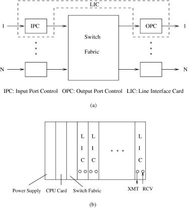
Figure 1.2Ža. depicts a typical ATM switch system model, consisting of input port controllers ŽIPCs., a switch fabric, and output port controllers ŽOPCs.. In practice, the IPC and the OPC are usually built on the same printed circuit board, called the line interface card ŽLIC.. Multiple IPCs and OPCs can be built on the same LIC. The center switch fabric provides interconnections between the IPCs and the OPCs. Figure 1.2Žb. shows a chasis containing a power supply card, a CPU card to perform operation, administration, and maintenance ŽOAM. functions for the switch system, a switch fabric card, and multiple LICs. Each LIC has a transmitter ŽXMT. and a receiver ŽRCV..

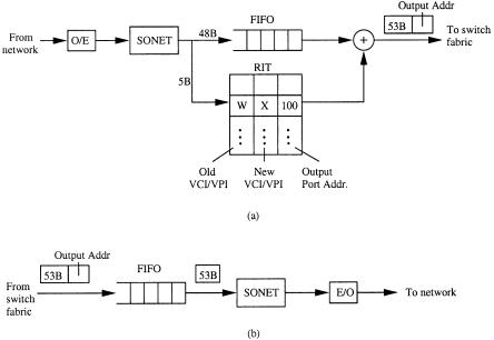
As shown in Figure 1.3Ža., each IPC terminates an incoming line and extracts cell headers for processing. In this example, optical signals are first converted to electrical signals by an optical-to-electrical ŽOrE. converter and then terminated by an SONET framer. Cell payloads are stored in a first-in, first-out ŽFIFO. buffer, while headers are extracted for routing processing. Incoming cells are aligned before being routed in the switch fabric, which greatly simplifies the design of the switch fabric. The cell stream is slotted, and the time required to transmit a cell across to the network is a time slot.

In Figure 1.3Žb., cells coming from the switch fabric are stored in a FIFO buffer.1 Routing information Žand other information such as a priority level,

1 For simplicity, here we use a FIFO for the buffer. To meet different QoS requirements for different connections, some kind of scheduling policies and buffer management schemes may be applied to the cells waiting to be transmitted to the output link. As a result, the buffer may not be as simple as a FIFO.

6INTRODUCTION

Fig. 1.2 An ATM switch system example.

if any. will be stripped off before cells are written to the FIFO. Cells are then carried in the payload of SONET frames, which are then converted to optical signals through an electrical-to-optical ŽErO. converter.

The OPC can transmit at most one cell to the transmission link in each time slot. Because cells arrive randomly in the ATM network, it is likely that more than one cell is destined for the same output port. This event is called output port contention Žor conflict.. One cell will be accepted for transmission, and the others must be either discarded or buffered. The location of the buffers not only affects the switch performance significantly, but also affects the switch implementation complexity. The choice of the contention resolution techniques is also influenced by the location of the buffers.

There are two methods of routing cells through an ATM switch fabric: self-routing and label routing. In self-routing, an output port address field Ž A. is prepended to each cell at the input port before the cell enters to the switch

Fig. 1.3 Input and output port controller block diagram.

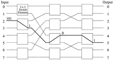
fabric. This field, which has log 2 N bits for unicast cells or N bits for multicastrbroadcast cells, is used to navigate the cells to their destination output ports. Each bit of the output port address field is examined by each stage of the switch element. If the bit is 0, the cell is routed to the upper output of the switch element. If the bit is 1, it is routed to its lower output. As shown in Figure 1.4, a cell whose output port address is 5 Ž101. is routed to input port 2. The first bit of the output port address Ž1. is examined by the first stage of the switch element. The cell is routed to the lower output and goes to the second stage. The next bit Ž0. is examined by the second stage, and the cell is routed to the upper output of the switch element. At the last stage of the switch element, the last bit Ž1. is examined and the cell is routed to its lower output, corresponding to output port 5. Once the cell arrives at the output port, the output port address is removed.

In contrast, in label routing the VPIrVCI field within the header is used by each switch module to make the output link decision. That is, each switch module has a VPIrVCI lookup table and switches cells to an output link according to the mapping between VPIrVCI and inputroutput links in the table. Label routing does not depend on the regular interconnection of switching elements as self-routing does, and can be used arbitrarily wherever switch modules are interconnected.

8INTRODUCTION

Fig. 1.4 An example of self-routing in a delta network.

1.2 IP ROUTER SYSTEMS

The Internet protocol corresponds to layer 3 as defined in the OSI reference model. The Internet, as originally conceived, offers best-effort data delivery. In contrast to ATM, which is a connection-oriented protocol, IP is a connectionless protocol. A user sends IP packets to IP networks without setting up any connection. As soon as a packet arrives at an IP router, the router decides to which output link the packet is to be routed, based on its IP address in the packet overhead, and transmits it to the output link.

To meet the demand for QoS for IP networks, the Internet Engineering Task Force ŽIETF. has proposed many service models and mechanisms, including the integrated servicesrresource reservation protocol ŽRSVP. model, the differentiated services ŽDS. model, MPLS, traffic engineering, and constraint-based routing w2x. These models will enhance today’s IP networks to support a variety of service applications.

1.2.1 Functions of IP Routers

IP routers’ functions can be classified into two categories, datapath functions and control functions w1x.

The datapath functions are performed on every datagram that passes through the router. These include the forwarding decision, switching through the backplane, and output link scheduling. When a packet arrives at the forwarding engine, its destination IP address is first masked by the subnet mask Žlogical AND operation., and the resulted address is used to look up the forwarding table. A so-called longest-prefix matching method is used to find the output port. In some application, packets are classified based on the combined information of IP sourcerdestination addresses, transport layer

port numbers Žsource and destination., and type of protocol: total 104 bits. Based on the result of classification, packets may be either discarded Žfirewall application. or handled at different priority levels. Then, the time-to-live ŽTTL. value is decremented and a new header checksum is calculated. Once the packet header is used to find an output port, the packet is delivered to the output port through a switch fabric. Because of contention by multiple packets destined for the same output port, packets are scheduled to be delivered to the output port in a fair manner or according to their priority levels.

The control functions include the system configuration, management, and exchange of routing table information. These are performed relatively infrequently. The route controller exchanges the topology information with other routers and constructs a routing table based on a routing protocol Že.g., RIP and OSPF.. It can also create a forwarding table for the forwarding engine. Since the control function is not processed for each arriving packet, it does not have a speed constraint and is implemented in software.

1.2.2 Architectures of IP Routers

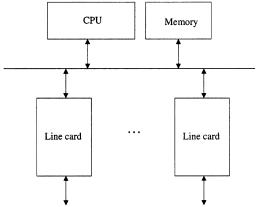
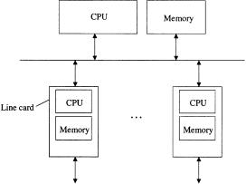
1.2.2.1 Low-End Routers In the architecture of the earliest routers, the forwarding decision and switching function were implemented in a central CPU with a shared central bus and memory, as shown in Figure 1.5. These functions are performed based on software. Since this software-based structure is cost-effective, it is mainly used by low-end routers. Although CPU performance has improved with time, it is still a bottleneck to handle all the packets transmitted through the router with one CPU.

Fig. 1.5 Low-end router structure.

10 INTRODUCTION

Fig. 1.6 Medium-size router structure.

1.2.2.2Middle-Size Routers To overcome the limitation of one central CPU, medium-size routers use router structure where each line card has a CPU and memory for packet forwarding, as shown in Figure 1.6. This structure reduces the central CPU load, because incoming packets are processed in parallel by the CPU associated with each line card, before they are sent through the shared bus to the central CPU and finally to the memory of the destined output line card. However, when the number of ports and the port speed increase, this structure still has a bottleneck at the central CPU and shared bus.

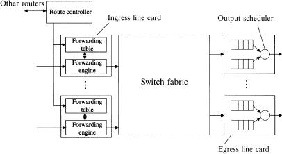
1.2.2.3High-End Routers In current high-performance routers, the forwarding engine is implemented in each associated ingress line card, and the switching function is implemented by using switch-fabric boards. As shown in Figure 1.7, a high-performance router consists of a route controller, forwarding engine, switch fabric, and output port scheduler. In this structure, multiple line cards can communicate with each other. Therefore, the router throughput is improved.

Once a packet is switched from an ingress line card to an egress line card, it is usually buffered at the output port that is implemented in the egress line card. This is because multiple packets may be destined for the same output port at the same time. Only one packet can be transmitted to the network at any time, and the rest of them must wait at the output buffer for the next transmission round. In order to provide differentiated service for different flows, it is necessary to schedule packets according to their priority levels or

the allocated bandwidth. There may also be some buffer management, such as random early detection ŽRED., to selectively discard packets to achieve certain goals Že.g., desynchronizing the TCP flows.. How to deliver packets from the forward engines to the output ports through the switch fabric is one of main topics to be discussed in this book.

Fig. 1.7 High-end router structure.

For high-performance routers, datapath functions are most often implemented in hardware. If any datapath function cannot be completed in the interval of the minimum packet length, the router will not be able to operate at so-called wire speed, nor accommodate all arriving shortest packets at the same time.

Packets can be transferred across the switch fabric in small fixed-size data units, or as variable-length packets. The fixed-size data units are called cells Žthey do not have to be the same length as in ATM, 53 bytes.. For the former case, each variable-length packet is segmented into cells at the input ports of the switch fabric and reassembled to that packet at the output ports. To design a high-capacity switch fabric, it is highly desirable to transfer packets in cells, for the following reasons. Due to output port contention, there is usually an arbiter to resolve contention among the input packets Žexcept for output-buffered switches, since all packets can arrive at the same output port simultaneously though, due to the memory speed constraint, the switch capacity is limited.. For the case of delivering cells across the switch fabric, scheduling is based on the cell time slot. At the beginning of a time slot, the arbiter will determine which inputs’ cells can be sent to the switch fabric. The arbitration process is usually overlapped Žor pipelined. with the cell transmission. That is, while cells that are arbitrated to be winners in last time slot are being sent through the switch fabric in the current time slot, the arbiter is scheduling cells for the next time slot. From the point of view of hardware implementation, it is also easier if the decision making, data transferring, and other functions are controlled in a synchronized manner, with cell time slots.

For the case of variable-length packets, there are two alternatives. In the first, as soon as an output port completely receives a packet from an input port, it can immediately receive another packet from any input ports that

12 INTRODUCTION

have packets destined for it. The second alternative is to transfer the packet in a cell-based fashion with the constraint that cells that belong to the same packet will be transmitted to the output port consecutively, and not interleaved with other cells. The differences between these two options have to do with event-driven vs. slot-driven arbitration. In the case of variable-length packets, the throughput is degraded, especially when supporting multicast services. Although the implementations of both alternatives are different, the basic cell transmission mechanisms are the same. Therefore, we describe an example of the variable-length-based operation by considering the first alternative for simplicity.

The first alternative starts the arbitration cycle as soon as a packet is completely transferred to the output port. It is difficult to have parallelism for arbitration and transmission, due to the lack of knowledge of when the arbitration can start. Furthermore, when a packet is destined for multiple output ports by taking advantage of the replication capability of the switch fabric Že.g., crossbar switch., the packet has to wait until all desired output ports become available. Consider a case where a packet is sent to output ports x and y. When output x is busy in accepting a packet from another input and output y is idle, the packet will not be able to send to output y until port x becomes available. As a result, the throughput for port y is degraded. However, if the packet is sent to port y without waiting for port x becomes available, as soon as port x becomes available, the packet will not be able to send to port x, since the remaining part of the packet is being sent to port y. One solution is to enable each input port to send multiple streams, which will increase the implementation complexity. However, if cell switching is used, the throughput degradation is only a cell slot time, as oppose to, when packet switching is used, the whole packet length, which can be a few tens or hundreds of cell slots.

1.2.2.4 Switch Fabric for High-End IP Routers Although most of today’s low-end to medium-size routers do not use switch fabric boards, high-end backbone IP routers will have to use the switch fabric as described in Section 1.2.2.3 in order to achieve the desired capacity and speed as the Internet traffic grows. In addition, since fixed-size cell-switching schemes achieve higher throughput and simpler hardware design, we will focus on the switch architecture using cell switching rather than packet switching.

Therefore, the high-speed switching technologies described in this book are common to both ATM switches and IP routers. The terms of packet switches and ATM switches are interchangeable. All the switch architectures discussed in this book deal with fixed-length data units. Variable-length packets in IP routers, Ethernet switches, and frame relay switches, are usually segmented into fixed-length data units Žnot necessarily 53 bytes like ATM cells. at the inputs. These data units are routed through a switch fabric and reassembled back to the original packets at the outputs.

Differences between ATM switches and IP routers systems lie in their line cards. Therefore, both ATM switch systems and IP routers can be constructed by using a common switch fabric with appropriate line cards.

1.3 DESIGN CRITERIA AND PERFORMANCE REQUIREMENTS

Several design criteria need to be considered when designing a packet switch architecture. First, the switch should provide bounded delay and small cell loss probability while achieving a maximum throughput close to 100%. Capability of supporting high-speed input lines is also an important criterion for multimedia services, such as video conferencing and videophone. Selfrouting and distributed control are essential to implement large-scale switches. Serving packets based on first come, first served provides correct packet sequence at the output ports. Packets from the same connection need to be served in sequence without causing out of order.

Bellcore has recommended performance requirements and objectives for broadband switching systems ŽBSSs. w3x. As shown in Table 1.1, three QoS classes and their associated performance objectives are defined: QoS class 1, QoS class 3, and QoS class 4. QoS class 1 is intended for stringent cell loss applications, including the circuit emulation of high-capacity facilities such as DS3. It corresponds to service class A, defined by ITU-T study group XIII. QoS class 3 is intended for low-latency, connection-oriented data transfer applications, corresponding to service class C in ITU-T study group XIII. QoS Class 4 is intended for low-latency, connectionless data transfer application, corresponding to service class D in ITU-T study group XIII.

The performance parameters used to define QoS classes 1, 3, and 4 are cell loss ratio, cell transfer delay, and two-point cell delay variation ŽCDV.. The values of the performance objectives corresponding to a QoS class depend on the status of the cell loss priority ŽCLP. bit ŽCLP s 0 for high

TABLE 1.1 Performance Objective across BSS for ATM Connections Delivering Cells to an STS-3c or STS-12c Interface

a NrS not specified.

b Includes nonqueuing related delays, excluding propagation. Does not include delays due to processing above ATM layer.

14 INTRODUCTION

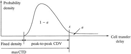
Fig. 1.8 Distribution of cell transfer delay.

priority, and CLP s 1 for low priority., which is initially set by the user and can be changed by a BSS within the connection’s path.

Figure 1.8 shows a typical distribution of the cell transfer delay through a switch node. The fixed delay is attributed to the delay of table lookup and other cell header processing, such as header error control ŽHEC. byte examination and generation. For QoS classes 1, 3, and 4, the probability of cell transfer delay ŽCTD. greater than 150 s is guaranteed to be less than

REFERENCES

1.N. McKeown, ‘‘A fast switched backplane for a gigabit switched router,’’ Business Commun. Re®., vol. 27, no. 12, Dec. 1997.

2.X. Xiao and L. M. Ni, ‘‘Internet QoS: a big picture,’’ IEEE Network, pp. 8 18, MarchrApril 1999.

3.Bellcore, ‘‘Broadband switching system ŽBSS. generic requirements, BSS performance,’’ GR-110-CORE, Issue 1, Sep. 1994.