height and frequency of breaking waves and the strength of the onshore wind. Rips are a danger to unwary swimmers, especially poor swimmers bobbing along in the waves inside the breaker zone. They are carried along by the along-shore current until they are suddenly carried out to sea by the rip. Swimming against the rip is futile, but swimmers can escape by swimming parallel to the beach.

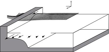
Edge waves are produced by the variability of wave energy reaching shore. Waves tend to come in groups, especially when waves come from distant storms. For several minutes breakers may be smaller than average, then a few very large waves will break. The minute-to-minute variation in the height of breakers produces low-frequency variability in the along-shore current. This, in turn, drives a low-frequency wave attached to the beach, an edge wave. The waves have periods of a few minutes, a long-shore wave length of around a kilometer, and an amplitude that decays exponentially o shore (figure 17.6).

z

x

y (north)

Figure 17.6 Computer-assisted sketch of an edge wave. Such waves exist in the breaker zone near the beach and on the continental shelf. After Cutchin and Smith (1973).

17.2Tsunamis

Tsunamis are low-frequency ocean waves generated by submarine earthquakes. The sudden motion of sea floor over distances of a hundred or more kilometers generates waves with periods of 15–40 minutes (figure 17.7). A quick calculation shows that such waves must be shallow-water waves, propagating at a speed of 180 m/s and having a wavelength of 130 km in water 3.6 km deep (figure 17.8). The waves are not noticeable at sea, but after slowing on approach to the coast, and after refraction by sub-sea features, they can come ashore and surge to heights ten or more meters above sea level. In an extreme example, the great 2004 Indian Ocean tsunami destroyed hundreds of villages, killing at least 200,000 people.

Shepard (1963, Chapter 4) summarized the influence of tsunamis based on his studies in the Pacific.

1.Tsunamis appear to be produced by movement (an earthquake) along a linear fault.

2.Tsunamis can travel thousands of kilometers and still do serious damage.

Figure 17.8 Tsunami waves four hours after the great M9 Cascadia earthquake o the coast of Washington on 26 January 1700 calculated by a finite-element, numerical model. Maximum open-ocean wave height, about one meter, is north of Hawaii. After Satake et al. (1996).

propagates the wave across ocean basins, and then calculates run-up when the wave comes ashore. It is initialized from a ground deformation model that uses measured earthquake magnitude and location to calculate vertical displacement of the sea floor. The forcing is modified once waves are measured near the earthquake by seafloor observing stations.

17.3Storm Surges

Storm winds blowing over shallow, continental shelves pile water against the coast. The increase in sea level is known as a storm surge. Several processes are important:

1.Ekman transport by winds parallel to the coast transports water toward the coast causing a rise in sea level.

2.Winds blowing toward the coast push water directly toward the coast.

3.Wave run-up and other wave interactions transport water toward the coast adding to the first two processes.

4.Edge waves generated by the wind travel along the coast.

5.The low pressure inside the storm raises sea level by one centimeter for each millibar decrease in pressure through the inverted-barometer e ect.

6.Finally, the storm surge adds to the tides, and high tides can change a relative weak surge into a much more dangerous one.

See Graber et al (2006) and §15.5 for a description of Advanced Circulation Model used by the National Hurricane Center for predicting storm-surges.

To a crude first approximation, wind blowing over shallow water causes a slope in the sea surface proportional to wind stress.

5.Earth’s crust is elastic. It bends under the influence of the tidal potential. It also bends under the weight of oceanic tides. As a result, the sea floor, and the continents move up and down by about 10 cm in response to the tides. The deformation of the solid earth influence almost all precise geodetic measurements.

6.Oceanic tides lag behind the tide-generating potential. This produces forces that transfer angular momentum between earth and the tide producing body, especially the moon. As a result of tidal forces, earth’s rotation about it’s axis slows, increasing the length of day; the rotation of the moon about earth slows, causing the moon to move slowly away from earth; and moon’s rotation about it’s axis slows, causing the moon to keep the same side facing earth as the moon rotates about earth.

7.Tides influence the orbits of satellites. Accurate knowledge of tides is needed for computing the orbit of altimetric satellites and for correcting altimeter measurements of oceanic topography.

8.Tidal forces on other planets and stars are important for understanding many aspects of solar-system dynamics and even galactic dynamics. For example, the rotation rate of Mercury, Venus, and Io result from tidal forces.

Mariners have known for at least four thousand years that tides are related to the phase of the moon. The exact relationship, however, is hidden behind many complicating factors, and some of the greatest scientific minds of the last four centuries worked to understand, calculate, and predict tides. Galileo, Descartes, Kepler, Newton, Euler, Bernoulli, Kant, Laplace, Airy, Lord Kelvin, Je reys, Munk and many others contributed. Some of the first computers were developed to compute and predict tides. Ferrel built a tide-predicting machine in 1880 that was used by the U.S. Coast Survey to predict nineteen tidal constituents. In 1901, Harris extended the capacity to 37 constituents.

Despite all this work important questions remained: What is the amplitude and phase of the tides at any place on the ocean or along the coast? What is the speed and direction of tidal currents? What is the shape of the tides on the ocean? Where is tidal energy dissipated? Finding answers to these simple questions is di cult, and the first, accurate, global maps of deep-sea tides were only published in 1994 (LeProvost et al. 1994). The problem is hard because the tides are a self-gravitating, near-resonant, sloshing of water in a rotating, elastic, ocean basin with ridges, mountains, and submarine basins.

Predicting tides along coasts and at ports is much easier. Data from a tide gauge plus the theory of tidal forcing gives an accurate description of tides near the tide gauge.

Tidal Potential Tides are calculated from the hydrodynamic equations for a self-gravitating ocean on a rotating, elastic earth. The driving force is the gradient of the gravity field of the moon and sun. If the earth were an ocean planet with no land, and if we ignore the influence of inertia and currents, the gravity gradient produces a pair of bulges of water on earth, one on the side

facing the moon or sun, one on the side away from the moon or sun. A clear derivation of the forces is given by Pugh (1987) and by Dietrich, Kalle, Krauss, and Siedler (1980). Here I follow the discussion in Pugh (1987: §3.2).

Note that many oceanographic books state that the tide is produced by two processes: i) the centripetal acceleration at earth’s surface as the earth and moon circle around a common center of mass, and ii) the gravitational attraction of mass on earth and the moon. However, the derivation of the tidal potential does not involve centripetal acceleration, and the concept is not used by the astronomical or geodetic communities.

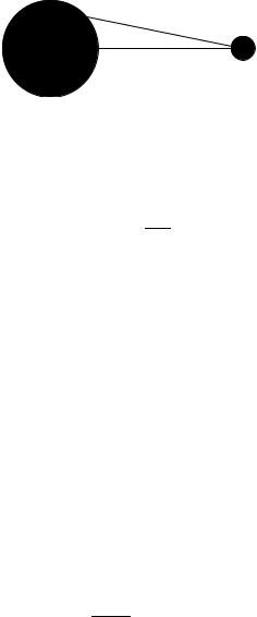
Figure 17.10 Sketch of coordinates for determining the tide-generating potential.

To calculate the amplitude and phase of the tide on an ocean planet, we begin by calculating the tide-generating potential. This is much easier than calculating the forces. Ignoring for now earth’s rotation, the rotation of moon about earth produces a potential VM at any point on earth’s surface

where the geometry is sketched in figure 17.10, γ is the gravitational constant, and M is moon’s mass. From the triangle OP A in the figure,

Using this in (17.5) gives

r/R ≈ 1/60, and (17.7) may be expanded in powers of r/R using Legendre polynomials (Whittaker and Watson, 1963: §15.1):

The tidal forces are calculated from the spatial gradient of the potential. The first term in (17.8) produces no force. The second term, when di erentiated with respect to (r cos ϕ) produces a constant force γM/R2 parallel to OA that keeps earth in orbit around the center of mass of the earth-moon system. The third term produces the tides, assuming the higher-order terms can be ignored. The tide-generating potential is therefore:

60 o

30 o

Z

0 o

-30 o

Figure 17.11 The horizontal component of the tidal force on earth when the tide-generating body is above the Equator at Z. After Dietrich et al. (1980: 413).

The tide-generating force can be decomposed into components perpendicular P and parallel H to the sea surface. Tides are produced by the horizontal component. “The vertical component is balanced by pressure on the sea bed, but the ratio of the horizontal force per unit mass to vertical gravity has to be balanced by an opposing slope of the sea surface, as well as by possible changes in current momentum” (Cartwright, 1999: 39, 45). The horizontal component, shown in figure 17.11, is:

The tidal potential is symmetric about the earth-moon line, and it produces symmetric bulges.

If we allow our ocean-covered earth to rotate, an observer in space sees the two bulges fixed relative to the earth-moon line as earth rotates. To an observer on earth, the two tidal bulges seems to rotate around earth because moon appears to move around the sky at nearly one cycle per day. Moon produces high tides every 12 hours and 25.23 minutes on the equator if the moon is above the equator. Notice that high tides are not exactly twice per day because the moon is also rotating around earth. Of course, the moon is above the equator only twice per lunar month, and this complicates our simple picture of the tides on an ideal ocean-covered earth. Furthermore, moon’s distance from earth R varies because moon’s orbit is elliptical and because the elliptical orbit is not fixed.

Clearly, the calculation of tides is getting more complicated than we might have thought. Before continuing on, we note that the solar tidal forces are derived in a similar way. The relative importance of the sun and moon are

nearly the same. Although the sun is much more massive than moon, it is much further away.

where Rsun is the distance to the sun, S is the mass of the sun, Rmoon is the distance to the moon, and M is the mass of the moon.

Coordinates of Sun and Moon Before we can proceed further we need to know the position of moon and sun relative to earth. An accurate description of the positions in three dimensions is very di cult, and it involves learning arcane terms and concepts from celestial mechanics. Here, I paraphrase a simplified description from Pugh (1987). See also figure 4.1.

A natural reference system for an observer on earth is the equatorial system described at the start of Chapter 3. In this system, declinations δ of a celestial body are measured north and south of a plane which cuts the earth’s equator.

Angular distances around the plane are measured relative to a point on this celestial equator which is fixed with respect to the stars. The point chosen for this system is the vernal equinox, also called the ‘First Point of Aries’. . . The angle measured eastward, between Aries and the equatorial intersection of the meridian through a celestial object is called the right ascension of the object. The declination and the right ascension together define the position of the object on a celestial background. . .

[Another natural reference] system uses the plane of the earth’s revolution around the sun as a reference. The celestial extension of this plane, which is traced by the sun’s annual apparent movement, is called the ecliptic. Conveniently, the point on this plane which is chosen for a zero reference is also the vernal equinox, at which the sun crosses the equatorial plane from south to north around 21 March each year. Celestial objects are located by their ecliptic latitude and ecliptic longitude. The angle between the two planes, of 23.45◦, is called the obliquity of the ecliptic. . . —Pugh (1987: 72).

Tidal Frequencies Now, let’s allow earth to spin about its polar axis. The changing potential at a fixed geographic coordinate on earth is:

where ϕp is latitude at which the tidal potential is calculated, δ is declination of moon or sun north of the equator, and τ1 is the hour angle of moon or sun. The hour angle is the longitude where the imaginary plane containing the sun or moon and earth’s rotation axis crosses the Equator.

The period of the solar hour angle is a solar day of 24 hr 0 m. The period of the lunar hour angle is a lunar day of 24 hr 50.47 m.

Earth’s axis of rotation is inclined 23.45◦ with respect to the plane of earth’s orbit about the sun. This defines the ecliptic, and the sun’s declination varies between δ = ±23.45◦ with a period of one solar year. The orientation of earth’s rotation axis precesses with respect to the stars with a period of 26 000 years. The rotation of the ecliptic plane causes δ and the vernal equinox to change slowly, and the movement called the precession of the equinoxes.

Earth’s orbit about the sun is elliptical, with the sun in one focus. That point in the orbit where the distance between the sun and earth is a minimum is called perigee. The orientation of the ellipse in the ecliptic plane changes slowly with time, causing perigee to rotate with a period of 20 942 years. Therefore Rsun varies with this period.

Moon’s orbit is also elliptical, but a description of moon’s orbit is much more complicated than a description of earth’s orbit. Here are the basics. The moon’s orbit lies in a plane inclined at a mean angle of 5.15◦ relative to the plane of the ecliptic. And lunar declination varies between δ = 23.45 ± 5.15◦ with a period of one tropical month of 27.32 solar days. The actual inclination of moon’s orbit varies between 4.97◦, and 5.32◦.

The shape of moon’s orbit also varies. First, perigee rotates with a period of 8.85 years. The eccentricity of the orbit has a mean value of 0.0549, and it varies between 0.044 and 0.067. Second, the plane of moon’s orbit rotates around earth’s axis of rotation with a period of 18.613 years. Both processes cause variations in Rmoon.

Note that I am a little imprecise in defining the position of the sun and moon. Lang (1980: § 5.1.2) gives much more precise definitions.

Substituting (17.15) into (17.9) gives:

V = γM3r2 1 3 sin2 ϕp − 1 3 sin2 δ − 1

R 4

+ 3 sin 2ϕp sin 2δ cos τ1

+ 3 cos2 ϕp cos2 δ cos 2τ1 (17.16)

Equation (17.16) separates the period of the lunar tidal potential into three terms with periods near 14 days, 24 hours, and 12 hours. Similarly the solar potential has periods near 180 days, 24 hours, and 12 hours. Thus there are three distinct groups of tidal frequencies: twice-daily, daily, and long period, having di erent latitudinal factors sin2 θ, sin 2θ, and (1 − 3 cos2 θ)/2, where θ is the co-latitude (90◦ − ϕ).

Doodson (1922) expanded (17.16) in a Fourier series using the cleverly chosen frequencies in table 17.1. Other choices of fundamental frequencies are possible, for example the local, mean, solar time can be used instead of the local, mean, lunar time. Doodson’s expansion, however, leads to an elegant decomposition of tidal constituents into groups with similar frequencies and spatial variability.

Using Doodson’s expansion, each constituent of the tide has a frequency