11.2. WESTERN BOUNDARY CURRENTS

Figure 11.6 Left: Mean annual wind stress Tx(y) over the Pacific and the curl of the wind stress. ϕb are the northern and southern boundaries of the gyres, where My = 0 and curl τ = 0. ϕ0 is the center of the gyre. Upper Right: The mass transport stream function for a rectangular basin calculated by Munk (1950) using observed wind stress for the Pacific. Contour interval is 10 Sverdrups. The total transport between the coast and any point x, y is ψ(x, y).The transport in the relatively narrow northern section is greatly exaggerated. Lower Right: North-South component of the mass transport. After Munk (1950).

is the biharmonic operator. Equation (11.18) is the same as (11.6) with the addition of the lateral friction term AH . The friction term is large close to a lateral boundary where the horizontal derivatives of the velocity field are large, and it is small in the interior of the ocean basin. Thus in the interior, the balance of forces is the same as that in Sverdrup’s solution.

Equation (11.18) is a fourth-order partial di erential equation, and four boundary conditions are needed. Munk assumed the flow at a boundary is parallel to a boundary and that there is no slip at the boundary:

where n is normal to the boundary. Munk then solved (11.18) with (11.20) assuming the flow was in a rectangular basin extending from x = 0 to x = r, and from y = −s to y = +s. He further assumed that the wind stress was zonal

Munk’s solution (figure 11.6) shows the dominant features of the gyre-scale circulation in an ocean basin. It has a circulation similar to Sverdrup’s in the eastern parts of the ocean basin and a strong western boundary current in the west. Using AH = 5 × 103 m2/s gives a boundary current roughly 225 km wide with a shape similar to the flow observed in the Gulf Stream and the Kuroshio.

The transport in western boundary currents is independent of AH , and it depends only on (11.6) integrated across the width of the ocean basin. Hence, it depends on the width of the ocean, the curl of the wind stress, and β. Using the best available estimates of the wind stress, Munk calculated that the Gulf Stream should have a transport of 36 Sv and that the Kuroshio should have a transport of 39 Sv. The values are about one half of the measured values of the flow available to Munk. This is very good agreement considering the wind stress was not well known.

Recent recalculations show good agreement except for the region o shore of Cape Hatteras where there is a strong recirculation. Munk’s solution was based on wind stress averaged aver 5◦squares. This underestimated the curl of the stress. Leetmaa and Bunker (1978) used modern drag coe cient and 2◦× 5◦ averages of stress to obtain 32 Sv transport in the Gulf Stream, a value very close to that calculated by Munk.

11.4Observed Surface Circulation in the Atlantic

The theories by Sverdrup, Munk, and Stommel describe an idealized flow. But the ocean is much more complicated. To see just how complicated the flow is at the surface, let’s look at a whole ocean basin, the north Atlantic. I have chosen this region because it is the best observed, and because mid-latitude processes in the Atlantic are similar to mid-latitude processes in the other ocean. Thus, for example, I use the Gulf Stream as an example of a western boundary current.

Let’s begin with the Gulf Stream to see how our understanding of ocean surface currents has evolved. Of course, we can’t look at all aspects of theflow. You can find out much more by reading Tomczak and Godfrey (1994) book onRegional Oceanography: An Introduction.

North Atlantic Circulation The north Atlantic is the most thoroughly studied ocean basin. There is an extensive body of theory to describe most aspects of the circulation, including flow at the surface, in the thermocline, and at depth, together with an extensive body of field observations. By looking at figures showing the circulation, we can learn more about the circulation, and by looking at the figures produced over the past few decades we can trace an ever more complete understanding of the circulation.

Let’s begin with the traditional view of the time-averaged surface flow in the north Atlantic based mostly on hydrographic observations of the density field

Figure 11.7 Sketch of the major surface currents in the North Atlantic. Values are transport in units of 106 m3/s. After Sverdrup, Johnson, and Fleming (1942: fig. 187).

(figure 2.7). It is a contemporary view of the mean circulation of the entire ocean based on a century of more of observations. Because the figure includes all the ocean, perhaps it is overly simplified. So, let’s look then at a similar view of the mean circulation of just the north Atlantic (figure 11.7).

The figure shows a broad, basin-wide, mid latitude gyre as we expect from Sverdrup’s theory described in §11.1. In the west, a western boundary current, the Gulf Stream, completes the gyre. In the north a subpolar gyre includes the Labrador current. An equatorial current system and countercurrent are found at low latitudes with flow similar to that in the Pacific. Note, however, the strong cross equatorial flow in the west which flows along the northeast coast of Brazil toward the Caribbean.

If we look closer at the flow in the far north Atlantic (figure 11.8) we see that the flow is still more complex. This figure includes much more detail of a region important for fisheries and commerce. Because it is based on an extensive base of hydrographic observations, is this reality? For example, if we were to drop a Lagrangian float into the Atlantic would it follow the streamline shown in the figure?

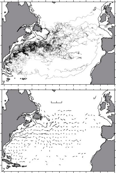
To answer the question, let’s look at the tracks of a 110 buoys drifting on the sea surface compiled by Phil Richardson (figure 11.9 top). The tracks give a very di erent view of the currents in the north Atlantic. It is hard to distinguish the flow from the jumble of lines, sometimes called spaghetti tracks. Clearly, the flow is very turbulent, especially in the Gulf Stream, a fast, western-boundary current. Furthermore, the turbulent eddies seem to have a diameter of a few degrees. This is much di erent than turbulence in the atmosphere. In the air, the large eddies are called storms, and storms have diameters of 10◦–20◦. Thus oceanic “storms” are much smaller than atmospheric storms.

Perhaps we can see the mean flow if we average the drifter tracks. What happens when Richardson averages the tracks through 2◦ × 2◦ boxes? The averages (figure 11.9 bottom) begin to show some trends, but note that in some

Figure 11.8 Detailed schematic of named currents in the north Atlantic. The numbers give the transport in units on 106m3/s from the surface to a depth of 1 km. Eg: East Greenland Current; Ei: East Iceland Current; Gu: Gulf Stream; Ir: Irminger Current; La: Labrador Current; Na: North Atlantic Current; Nc: North Cape Current; Ng: Norwegian Current; Ni: North Iceland Current; Po: Portugal Current; Sb: Spitsbergen Current; Wg: West Greenland Current. Numbers within squares give sinking water in units on 106m3/s. Solid Lines: Warmer currents. Broken Lines: Colder currents. After Dietrich et al. (1980: 542).

regions, such as east of the Gulf Stream, adjacent boxes have very di erent means, some having currents going in di erent directions. This indicates the flow is so variable, that the average is not stable. Forty or more observations do not yields a stable mean value. Overall, Richardson finds that the kinetic energy of the eddies is 8 to 37 times larger than the kinetic energy of the mean flow. Thus oceanic turbulence is very di erent than laboratory turbulence. In the lab, the mean flow is typically much faster than the eddies.

Further work by Richardson (1993) based on subsurface buoys freely drifting at depths between 500 and 3,500 m, shows that the current extends deep below the surface, and that typical eddy diameter is 80 km.

Gulf Stream Recirculation Region If we look closely at figure 11.7 we see that the transport in the Gulf Stream increases from 26 Sv in the Florida Strait (between Florida and Cuba) to 55 Sv o shore of Cape Hatteras. Later measurements showed the transport increases from 30 Sv in the Florida Strait to 150 Sv near 40◦N.

The observed increase, and the large transport o Hatteras, disagree with transports calculated from Sverdrup’s theory. Theory predicts a much smaller