

Chapter 10
Geostrophic Currents
Within the ocean’s interior away from the top and bottom Ekman layers, for horizontal distances exceeding a few tens of kilometers, and for times exceeding a few days, horizontal pressure gradients in the ocean almost exactly balance the Coriolis force resulting from horizontal currents. This balance is known as the geostrophic balance.
The dominant forces acting in the vertical are the vertical pressure gradient and the weight of the water. The two balance within a few parts per million. Thus pressure at any point in the water column is due almost entirely to the weight of the water in the column above the point. The dominant forces in the horizontal are the pressure gradient and the Coriolis force. They balance within a few parts per thousand over large distances and times (See Box).
Both balances require that viscosity and nonlinear terms in the equations of motion be negligible. Is this reasonable? Consider viscosity. We know that a rowboat weighing a hundred kilograms will coast for maybe ten meters after the rower stops. A super tanker moving at the speed of a rowboat may coast for kilometers. It seems reasonable, therefore that a cubic kilometer of water weighing 1015 kg would coast for perhaps a day before slowing to a stop. And oceanic mesoscale eddies contain perhaps 1000 cubic kilometers of water. Hence, our intuition may lead us to conclude that neglect of viscosity is reasonable. Of course, intuition can be wrong, and we need to refer back to scaling arguments.
10.1Hydrostatic Equilibrium
Before describing the geostrophic balance, let’s first consider the simplest solution of the momentum equation, the solution for an ocean at rest. It gives the hydrostatic pressure within the ocean. To obtain the solution, we assume the fluid is stationary:
|
u = v = w = 0; |
(10.1) |
|||||
the fluid remains stationary: |
|
|
|
|
|
|
|
|
du |
= |
dv |
= |
dw |
= 0; |
(10.2) |
|
dt |
dt |
dt |
||||
|
|
|
|
|
|||
151

152 CHAPTER 10. GEOSTROPHIC CURRENTS
Scaling the Equations: The Geostrophic Approximation
We wish to simplify the equations of motion to obtain solutions that describe the deep-sea conditions well away from coasts and below the Ekman boundary layer at the surface. To begin, let’s examine the typical size of each term in the equations in the expectation that some will be so small that they can be dropped without changing the dominant characteristics of the solutions. For interior, deep-sea conditions, typical values for distance L, horizontal velocity U , depth H, Coriolis
parameter f , gravity g, and density ρ are: |
|
|||
L ≈ 106 m |
H1 |
≈ 103 m |
f ≈ 10−4 s−1 |
ρ ≈ 103 kg/m3 |
U ≈ 10−1 m/s |
H2 |
≈ 1 m |
ρ ≈ 103 kg/m3 |
g ≈ 10 m/s2 |
where H1 and H2 are typical depths for pressure in the vertical and horizontal. From these variables we can calculate typical values for vertical velocity W ,
pressure P , and time T : |
|
|
|
|
|
|
|
|
|
|
|
|
|
|
|
|
|
|
|
|
|||||||||||||||
|
∂W |
„ |
∂U |
∂v |
« |
|
|
|
|
|
|
|
|
|
|
|
|
|
|
|
|||||||||||||||
|
|
|
= − |
|
|
+ |
|
|
|
|
|
|
|
|
|
|
|
|
|
|
|
|
|
|
|
||||||||||
|
∂z |
∂x |
∂y |
|
|
|
|
|
|
|
|
|
|
|
|
|
|
|
|||||||||||||||||
|
|
W U |
|
|
|
|
|
|
|
|
U H1 |
|
|
10−1 103 |
|
|
|
|
|
|
−4 |
|
|||||||||||||
|
|
|
= |
|
|
|
; |
W = |
|
|
|
|
|
= |
|
|
|
|
|
|
m/s = 10 |
m/s |
|||||||||||||
|
|
H1 |
L |
L |
|
|
|
|
106 |
|
|||||||||||||||||||||||||
|
|
P = ρgH1 = 103 101 103 = 107 Pa; |
∂p/∂x = ρgH2/L = 10−2 Pa/m |
||||||||||||||||||||||||||||||||
|
|
T = L/U = 107 s |
|
|
|
|
|
|
|
|
|
|
|
|
|
|
|
|
|
|
|||||||||||||||
The momentum equation for vertical velocity is therefore: |
|||||||||||||||||||||||||||||||||||
|
|
|
|
∂w |
|
+ u |
∂w |
|
+ v |
∂w |
|
+ w |
∂w |
|
= − |
1 |
|
∂p |
+ 2Ω u cos ϕ − g |
||||||||||||||||
|
|
|
|
∂t |
∂x |
∂y |
∂z |
|
|
|
|||||||||||||||||||||||||
|
|
|
|
|
|
|
|
|
|
|
|
|
|
|
|
|
|
|
ρ ∂z |
|
|||||||||||||||
|
|
|
|
|
W |
|
+ |
U W |
|
+ |
|
U W |
|
+ |
|
W 2 |
|
= |
P |
|
|
+ f U − g |
|||||||||||||
|
|
|
|
|
|
T |
|
|
|
|
|
L |
|
|
H |
|
|
|
|||||||||||||||||
|
|
|
|
|
|
|
|
|
|
|
L |
|
|
|
|
|
|
|
|
|
ρ H1 |
|
|||||||||||||
|
|
|
10−11 + 10−11 + 10−11 + 10−11 = 10 |
|
|
+ 10−5 − 10 |
|||||||||||||||||||||||||||||
and the only important balance in the vertical is hydrostatic: |
|||||||||||||||||||||||||||||||||||
|
|
|
|
|
|
|
|
|
|
|
|
|
|
|
|
∂p |
|
|
|
|
|
|
|
|
|
|
|
|
|
|
|
|
|
6 |
|
|
|
|
|
|
|
|
|
|
|
|
|
|
|
|
|
|
|
= −ρg |
Correct to |
1 : 10 . |
|||||||||||||||
|
|
|
|
|
|
|
|
|
|
|
|
|
|
|
|
∂z |
|||||||||||||||||||
The momentum equation for horizontal velocity in the x direction is:
|
∂u |
+ u |
∂u |
+ v |
∂u |
+ w |
∂u |
= − |
1 ∂p |
+ f v |
||
|
|
|
|
|
|
|
|
|||||
|
∂t |
∂x |
∂y |
∂z |
ρ ∂x |
|||||||
|
|
|
|
|
|
|||||||
10−8 + 10−8 + 10−8 + 10−8 = 10−5 + 10−5 |
||||||||||||
Thus the Coriolis force balances the pressure gradient within one part per thousand. This is called the geostrophic balance, and the geostrophic equations are:
|
1 ∂p |
= f v; |
1 ∂p |
= −f u; |
1 ∂p |
= −g |
|||||||
|
|
|
|
|
|
|
|
|
|
|
|||
|
ρ ∂x |
ρ ∂y |
ρ ∂z |
||||||||||
|
|
|
|
||||||||||
This balance applies to |
oceanic |
flows |
with horizontal dimensions larger than |
||||||||||
roughly 50 km and times greater than a few days.
10.2. GEOSTROPHIC EQUATIONS |
|
|
|
|
153 |
|||||||||
and, there is no friction: |
|
|
|
|
|
|
|
|
|
|
||||
|
|
|
|
|
fx = fy = fz = 0. |
|
|
|
|
(10.3) |
||||
With these assumptions the momentum equation (7.12) becomes: |
|
|||||||||||||
|
1 ∂p |
|
1 ∂p |
1 ∂p |
|
|
||||||||
|
|
|
|
= 0; |
|
|
|
|
= 0; |
|
|
|
= − g(ϕ, z) |
(10.4) |
|
ρ |
∂x |
ρ |
∂y |
ρ ∂z |
|||||||||
where I have explicitly noted that gravity g is a function of latitude ϕ and height z. I will show later why I have kept this explicit.
Equations (10.4) require surfaces of constant pressure to be level surface (see page 30). A surface of constant pressure is an isobaric surface. The last equation can be integrated to obtain the pressure at any depth h. Recalling that ρ is a function of depth for an ocean at rest.
|
Z 0 |
|
p = |
g(ϕ, z) ρ(z) dz |
(10.5) |
−h
For many purposes, g and ρ are constant, and p = ρ g h. Later, I will show that (10.5) applies with an accuracy of about one part per million even if the ocean is not at rest.
The SI unit for pressure is the pascal (Pa). A bar is another unit of pressure. One bar is exactly 105 Pa (table 10.1). Because the depth in meters and pressure in decibars are almost the same numerically, oceanographers prefer to state pressure in decibars.
Table 10.1 Units of Pressure
1 pascal (Pa) |
= |
1 N/m2 = 1 kg·s−2·m−1 |
|
1 bar |
= |
105 |
Pa |
1 decibar |
= |
104 |
Pa |
1 millibar |
= |
100 Pa |
|
10.2Geostrophic Equations
The geostrophic balance requires that the Coriolis force balance the horizontal pressure gradient. The equations for geostrophic balance are derived from the equations of motion assuming the flow has no acceleration, du/dt = dv/dt = dw/dt = 0; that horizontal velocities are much larger than vertical, w u, v; that the only external force is gravity; and that friction is small. With these assumptions (7.12) become
∂p |
= ρf v; |
∂p |
= −ρf u; |
∂p |
= −ρg |
(10.6) |
|
|
|
||||
∂x |
∂y |
∂z |
where f = 2Ω sin ϕ is the Coriolis parameter. These are the geostrophic equations.
The equations can be written: |
|
|
|
|
|
|
|||
u = − |
1 ∂p |
; |
v = |
1 ∂p |
(10.7a) |
||||
|
|
|
|
|
|
||||
f ρ |
∂y |
f ρ ∂x |
|||||||
154 |
CHAPTER 10. GEOSTROPHIC CURRENTS |
||
|
p = p0 |
+ Z−h g(ϕ, z)ρ(z)dz |
(10.7b) |
|
|
ζ |
|
where p0 is atmospheric pressure at z = 0, and ζ is the height of the sea surface. Note that I have allowed for the sea surface to be above or below the surface z = 0; and the pressure gradient at the sea surface is balanced by a surface current us.
Substituting (10.7b) into (10.7a) gives:
1 |
|
∂ |
|
u = − |
|
|
|
f ρ |
∂y |
||
1 |
|
∂ |
|
u = −f ρ ∂y
Z−h g(ϕ, z) ρ(z) dz − f ∂y |
||
0 |
g |
∂ζ |
Z−h g(ϕ, z) ρ(z) dz − us |
(10.8a) |
|
0 |
|
|
where I have used the Boussinesq approximation, retaining full accuracy for ρ only when calculating pressure.
In a similar way, we can derive the equation for v.
v = f1ρ ∂x |
Z−h g(ϕ, z) ρ(z) dz + f ∂x |
|||||
|
|
|
∂ |
0 |
g |
∂ζ |
v = f1ρ ∂x |
Z−h g(ϕ, z) ρ(z) dz + vs |
(10.8b) |
||||
|
|
|
∂ |
0 |
|
|
If the ocean is homogeneous and density and gravity are constant, the first term on the right-hand side of (10.8) is equal to zero; and the horizontal pressure gradients within the ocean are the same as the gradient at z = 0. This is barotropic flow described in §10.4.
If the ocean is stratified, the horizontal pressure gradient has two terms, one due to the slope at the sea surface, and an additional term due to horizontal density di erences. These equations include baroclinic flow also discussed in §10.4. The first term on the right-hand side of (10.8) is due to variations in density ρ(z), and it is called the relative velocity. Thus calculation of geostrophic currents from the density distribution requires the velocity (u0, v0) at the sea surface or at some other depth.
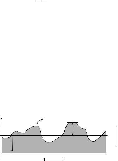
z |
Sea Surface (z = ζ) |
|
|
|
|
|
ζ |
|
0 |
x |
1m |
z=-r
-r
100km
Figure 10.1 Sketch defining ζ and r, used for calculating pressure just below the sea surface.