


14.1. EQUATORIAL PROCESSES |
237 |
Average Velocity at 10 m Jan 1981 – Dec 1994
20 o |
|
|
|
|
|
|
|
10 o |
|
|
|
|
|
|
|
0 o |
|
|
|
|
|
|
|
-10 o |
|
|
|
|
|
|
|
-20 o |
|
|
|
20.0 cm/s |
|
|
|
|
|
|
|
|
|
||
140 o |
160 o |
180 o |
-160 o |
-140 o |
-120 o |
-100 o |
-80 o |
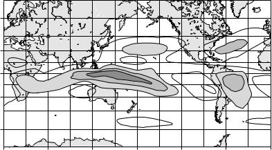
Figure 14.3 Average currents at 10 m calculated from the Modular Ocean Model driven by observed winds and mean heat fluxes from 1981 to 1994. The model, operated by the noaa National Centers for Environmental Prediction, assimilates observed surface and subsurface temperatures. After Behringer, Ji, and Leetmaa (1998).
Surface Currents The strong stratification confines the wind-driven circulation to the mixed layer and upper thermocline. Sverdrup’s theory and Munk’s extension, described in §11.1 and §11.3, explain the surface currents in the tropical Atlantic, Pacific, and Indian ocean. The currents include (figure 14.3):
1.The North Equatorial Countercurrent between 3◦N and 10◦N, which flows eastward with a typical surface speed of 50 cm/s. The current is centered on the band of weak winds, the doldrums, around 5–10◦N where the north and south trade winds converge, the tropical convergence zone.
2.The North and South Equatorial Currents which flow westward in the zonal band on either side of the countercurrent. The currents are shallow, less than 200 m deep. The northern current is weak, with a speed less than roughly 20 cm/s. The southern current has a maximum speed of around 100 cm/s, in the band between 3◦N and the equator.
The currents in the Atlantic are similar to those in the Pacific because the trade winds in that ocean also converge near 5◦–10◦N. The South Equatorial Current in the Atlantic continues northwest along the coast of Brazil, where it is known as the North Brazil Current. In the Indian Ocean, the doldrums occur in the southern hemisphere and only during the northern-hemisphere winter. In the northern hemisphere, the currents reverse with the monsoon winds.
There is, however, much more to the story of equatorial currents.
Equatorial Undercurrent: Observations Just a few meters below the surface on the equator is a strong eastward flowing current, the Equatorial Undercurrent, the last major oceanic current to be discovered. Here’s the story:
In September 1951, aboard the U.S. Fish and Wildlife Service research vessel long-line fishing on the equator south of Hawaii, it was noticed that the subsurface gear drifted steadily to the east. The next year Cromwell, in company with Montgomery and Stroup, led an expedition to investigate the vertical distribution of horizontal velocity at the equator. Using
238 |
CHAPTER 14. EQUATORIAL PROCESSES |
floating drogues at the surface and at various depths, they were able to establish the presence, near the equator in the central Pacific, of a strong, narrow eastward current in the lower part of the surface layer and the upper part of the thermocline (Cromwell, et. al., 1954). A few years later the Scripps Eastropac Expedition, under Cromwell’s leadership, found the current extended toward the east nearly to the Galapagos Islands but was not present between those islands and the South American continent.
The current is remarkable in that, even though comparable in transport to the Florida Current, its presence was unsuspected ten years ago. Even now, neither the source nor the ultimate fate of its waters has been established. No theory of oceanic circulation predicted its existence, and only now are such theories being modified to account for the important features of its flow.—Warren S. Wooster (1960).
The Equatorial Undercurrent in the Atlantic was first discovered by Buchanan in 1886, and in the Pacific by the Japanese Navy in the 1920s and 1930s (McPhaden, 1986).
However, no attention was paid to these observations. Other earlier hints regarding this undercurrent were mentioned by Matth¨aus (1969). Thus the old experience becomes even more obvious which says that discoveries not attracting the attention of contemporaries simply do not exist.— Dietrich et al. (1980).
Bob Arthur (1960) summarized the major aspects of the flow:
1.Surface flow may be directed westward at speeds of 25–75 cm/s;
2.Current reverses at a depth of from 20 to 40 m;
3.Eastward undercurrent extends to a depth of 400 meters with a transport of as much as 30 Sv = 30 × 106 m3/s;
4.Core of maximum eastward velocity (0.50–1.50 m/s) rises from a depth of 100 m at 140◦W to 40 m at 98◦W, then dips down;
5.Undercurrent appears to be symmetrical about the equator and becomes much thinner and weaker at 2◦N and 2◦S.
In essence, the Pacific Equatorial Undercurrent is a ribbon with dimensions of 0.2 km × 300 km × 13, 000 km (figure 14.4).
Equatorial Undercurrent: Theory Although we do not yet have a complete theory for the undercurrent, we do have a clear understanding of some of the more important processes at work in the equatorial regions. Pedlosky(1996), in his excellent chapter on Equatorial Dynamics of the Thermocline: The Equatorial Undercurrent, points out that the basic dynamical balances we have used in mid latitudes break down near or on the equator.
Near the equator:
1. The Coriolis parameter becomes very small, going to zero at the equator:
f = 2Ω sin ϕ = βy ≈ 2Ω ϕ |
(14.1) |
where ϕ is latitude, β = ∂f /∂y ≈ 2Ω/R near the equator, and y = R ϕ.
14.1. EQUATORIAL PROCESSES |
239 |
|
0 |
0 |
|
|
|
|
|
|
|
|
|
|
|
|
|
|
|
0 |
|
|
|
|
|
|
|
|
|
|
|
|
-100 |
|
|
20 |
|
|
|
20 |
|
|
|
|
|
|
|
10 |
|
|
|
(m) |
|
|
|
|
|
|
|
|
|
-200 |
|
0 |
|
|
|
|
|
|
|
|
|
10 |
|
|
10 |
|
|
||
Depth |
|
|
|
50 |
|
|
|
||
|
|
|
|
|
0 |
|
|
||
-300 |
|
|
|
30 |
|
|
|
|
|
|
|
|
|
|
|
|
|
||
|
-400 |
|
|
0 |
10 |
0 |
|
|
|
|
|
|
0 |
|
|
|
u (cm/s) |
||
|
|
0 |
|
|
|
|
|
||
|
-500 |
|
|
|
|
|
|
|
|
|
|
|
|
|
|
|
|
|
|
|
|
-15 o |
-10 o |
- 5 o |
0 o |
5 o |
10 o |
|
15 o |
|
0 |
28.0 |
|
|
|
|
|
|
|
|
|
|
|
|
|
|
|
||
|
-100 |
26.0 |
|
|
|
|
|
|
|
|
24.0 |
|
|
|
|
|
|
||
(m) |
|
|
|
|
|
|
|
||
-200 |
22.0 |
|
|
|
|
|
|
||
|
20.0 |
|
|
|
|
|
|
||
Depth |
|
|
18.0 |
|
|
|
|
|
|
-300 |
|
.0 |
|
|
|
|
|
|
|
|
16 |
|
|
|
|
|
|
||
|
|
.0 |
|
|
|
|
|
|
|
|
|
|
14 |
|
|
|
|
|
|
|
|
|
.0 |
|
|
|
|
|
|
|
-400 |
|
12 |
|
|
|
|
|
t (Celsius) |
|
|
10.0 |
|
|
|
|
|
||
|
|
|
|
|
|
|
|
||
|
-500 |
|
|
|
|
|
|
|
|
|
|
-15 o |
-10 o |
- 5 o |
0 o |
5 o |
10 o |
|
15 o |
|
0 |
|
|
|
|
|
|
.60 |
|
|
|
|
|
|
|
|
|
|
|
|
|
|
|
|
|
|
|
34 |
|
|
-100 |
|
|
|
|
|
|
|
|
(m) |
-200 |
|
|
|
|
|
|
|
34. |
Depth |
|
|
.60 |
|
|
|
|
|
80 |
-300 |
35 |
|
|
|
|
|
|
||
35.40 |
|
|
|
|
34 |
|
|||
|
|
|
|
|
|
|
. |
||
|
|
|
35.20 |
|
|
|
|
|
60 |
|
-400 |
|
|
|
|
|
|
|
|
|
|
35.00 |
|
34.80 |
|
|
|
|
|
|
|
|
|
|
|
|
S |
||
|
|
|
|
|
|
|
|
|
|
|
-500 |
|
|
|
|
|
|
|
|
|
|
-15 o |
-10 o |
- 5 o |
0 o |
5 o |
10 o |
|
15 o |
|
|
|
|
|
Latitude |
|
|
|
|
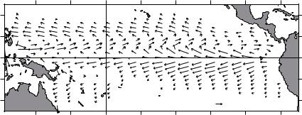
Figure 14.4 Cross section of the Equatorial Undercurrent in the Pacific calculated from Modular Ocean Model with assimilated surface data (See §14.5). The section is an average from 160◦E to 170◦E from January 1965 to December 1999. Stippled areas are westward flowing. From Nevin S. Fuˇckar.
2. Planetary vorticity f is also small, and the advection of relative vorticity cannot be neglected. Thus the Sverdrup balance (11.7) must be modified.
3. The geostrophic and vorticity balances fail when the meridional distance
p
L to the equator is O U/β , where β = ∂f /∂y. If U = 1 m/s, then
L = 200 km or 2◦ of latitude. Lagerloe et al (1999), using measured currents, show that currents near the equator can be described by the geostrophic balance for |ϕ| > 2.2◦. They also show that flow closer to the equator can be described using a β-plane approximation f = βy.
4.The geostrophic balance for zonal currents works so well near the equator because f and ∂ζ/∂y → 0 as ϕ → 0, where ζ is sea surface topography.
Upwelled water along the equator produced by Ekman pumping is not part of a two-dimensional flow in a north-south, meridional plane. The flow is threedimensional. Water tends to flow along the contours of constant density (isopycnal surfaces), close to the lines of constant temperature in figure 14.2. Cold water enters the undercurrent in the far west Pacific, and it moves eastward

˜ |
241 |
14.2. EL NINO |
A Little History In the 19th century, the term was applied to conditions o the coast of Peru. The following quote comes from the introduction to Philander’s (1990) excellent book El Ni˜no, La Ni˜na, and the Southern Oscillation:
In the year 1891, Se˜nor Dr. Luis Carranza of the Lima Geographical Society, contributed a small article to the Bulletin of that Society, calling attention to the fact that a counter-current flowing from north to south had been observed between the ports of Paita and Pacasmayo.
The Paita sailors, who frequently navigate along the coast in small craft, either to the north or the south of that port, name this countercurrent the current of “El Ni˜no” (the Child Jesus) because it has been observed to appear immediately after Christmas.
As this counter-current has been noticed on di erent occasions, and its appearance along the Peruvian coast has been concurrent with rains in latitudes where it seldom if ever rains to any great extent, I wish, on the present occasion, to call the attention of the distinguished geographers here assembled to this phenomenon, which exercises, undoubtedly, a very great influence over the climatic conditions of that part of the world.— Se˜nor Frederico Alfonso Pezet’s address to the Sixth International Geographical Congress in Lima, Peru 1895.
The Peruvians noticed that in some years the El Ni˜no current was stronger than normal, it penetrated further south, and it is associated with heavy rains in Peru. This occurred in 1891 when (again quoting from Philander’s book)
. . . it was then seen that, whereas nearly every summer here and there there is a trace of the current along the coast, in that year it was so visible, and its e ects were so palpable by the fact that large dead alligators and trunks of trees were borne down to Pacasmayo from the north, and that the whole temperature of that portion of Peru su ered such a change owing to the hot current that bathed the coast. . . . —Se˜nor Frederico Alfonso Pezet.
. . . the sea is full of wonders, the land even more so. First of all the desert becomes a garden . . . . The soil is soaked by the heavy downpour, and within a few weeks the whole country is covered by abundant pasture. The natural increase of flocks is practically doubled and cotton can be grown in places where in other years vegetation seems impossible.—From Mr. S.M. Scott & Mr. H. Twiddle quoted from a paper by Murphy, 1926.
The El Ni˜no of 1957 was even more exceptional. So much so that it attracted the attention of meteorologists and oceanographers throughout the Pacific basin.
By the fall of 1957, the coral ring of Canton Island, in the memory of man ever bleak and dry, was lush with the seedlings of countless tropical trees and vines.
One is inclined to select the events of this isolated atoll as epitomizing the year, for even here, on the remote edges of the Pacific, vast concerted shifts in the ocean and atmosphere had wrought dramatic change.
Elsewhere about the Pacific it also was common knowledge that the year had been one of extraordinary climatic events. Hawaii had its first recorded typhoon; the seabird-killing El Ni˜no visited the Peruvian coast;

˜ |
243 |
14.2. EL NINO |
Normalized Southern Oscillation Index
|
3 |
|
|
|
|
|
|
|
|
|
|
|
2 |
|
|
|
|
|
|
|
|
|
|
Index |
1 |
|
|
|
|
|
|
|
|
|
|
|
|
|
|
|
|
|
|
|
|
|
|
Normalized |
0 |
|
|
|
|
|
|
|
|
|
|
-1 |
|
|
|
|
|
|
|
|
|
|
|
-2 |
|
|
|
|
|
|
|
|
|
|
|
|
-3 |
|
|
|
|
|
|
|
|
|
|
|
-4 |
|
|
|
|
|
|
|
|
|
|
|
1950 |
1955 |
1960 |
1965 |
1970 |
1975 |
1980 |
1985 |
1990 |
1995 |
2000 |
|
|
|
|
|
|
Date |
|
|
|
|
|
Figure 14.7 Normalized Southern Oscillation Index from 1951 to 1999. The normalized index is sea-level pressure anomaly at Tahiti divided by its standard deviation minus sea-level pressure anomaly at Darwin divided by its standard deviation then the di erence is divided by the standard deviation of the di erence. The means are calculated from 1951 to 1980. Monthly values of the index have been smoothed with a 5-month running mean. Strong El Ni˜no events occurred in 1957–58, 1965–66, 1972–73, 1982–83, 1997–98. Data from noaa.
The connection between the Southern Oscillation and El Ni˜no was made soon after the Rancho Santa Fe meeting. Ichiye and Petersen (1963) and Bjerknes (1966) noticed the relationship between equatorial temperatures in the Pacific during the 1957 El Ni˜no and fluctuations in the trade winds associated with the Southern Oscillation. The theory was further developed by Wyrtki (1975).
Because El Ni˜no and the Southern Oscillation are so closely related, the phenomenon is often referred to as the El Ni˜no–Southern Oscillation or enso. More recently, the oscillation is referred to as El Ni˜no/La Ni˜na, where La Ni˜na refers to the positive phase of the oscillation when trade winds are strong, and water temperature in the eastern equatorial region is very cold.
Definition of El Ni˜no Philander (1990) points out that each El Ni˜no is unique, with di erent temperature, pressure, and rainfall patterns. Some are strong, some are weak. So, exactly what events deserve to be called El Ni˜no? The icoads data show that the best indicator of El Ni˜no is sea-level pressure anomaly in the eastern equatorial Pacific from 4◦S to 4◦N and from 108◦W to 98◦W (Harrison and Larkin, 1996). It correlates better with sea-surface temperature in the central Pacific than with the Southern-Oscillation Index. Thus the importance of the El Ni˜no is not exactly proportional to the Southern Oscillation Index—the strong El Ni˜no of 1957–58, has a weaker signal in figure 14.7 than the weaker El Ni˜no of 1965–66.
Trenberth (1997) recommends that those disruptions of the equatorial system in the Pacific shall be called an El Ni˜no only when the 5-month running mean of sea-surface temperature anomalies in the region 5◦N–5◦S, 120◦W– 170◦W exceeds 0.4◦C for six months or longer.
So El Ni˜no, which started life as a change in currents o Peru each Christmas, has grown into a giant. It now means a disruption of the ocean-atmosphere system over the whole equatorial Pacific.

246 |
CHAPTER 14. EQUATORIAL PROCESSES |
A complete El Ni˜no cycle results in a net heat discharge from the tropical Pacific toward higher latitudes. At the end of the cycle the tropical Pacific is depleted of heat, which can only be restored by the slow accumulation of warm water in the western Pacific by the normal trade winds. Consequently, the time scale of the Southern Oscillation is given by the time required for the accumulation of warm water in the western Pacific.
It is these far reaching events that make El Ni˜no so important. Few people care about warm water o Peru around Christmas, many care about global changes the weather. El Ni˜no is important because of its atmospheric influence.
When the Kelvin wave reaches the coast of Ecuador, part is reflected as an westward propagating Rossby wave, and part propagates north and south as a coastal trapped Kelvin wave carrying warm water to higher latitudes. For example, during the 1957 El Ni˜no, the northward propagating Kelvin wave produced unusually warm water o shore of California, and it eventually reached Alaska. This warming of the west coast of North America further influences climate in North America, especially in California.
As the Kelvin wave moves along the coast, it forces Rossby waves which move west across the Pacific at a velocity that depends on the latitude (14.4). The velocity is very slow at high latitudes and fastest on the equator, where the reflected wave moves back as a deepening of the thermocline, reaching the central equatorial Pacific a year later. Similarly, the westward propagating Rossby wave launched at the start of the El Ni˜no in the west, reflects o Asia and returns to the central equatorial Pacific as a Kelvin wave, again about a year later.
El Ni˜no ends when the Rossby waves reflected from Asia and Ecuador meet in the central Pacific about a year after the onset of El Ni˜no (Picaut, Masia, and du Penhoat, 1997). The waves push the warm pool at the surface toward the west. At the same time, the Rossby wave reflected from the western boundary causes the thermocline in the central Pacific to become shallower when the waves reaches the central Pacific. Then any strengthening of the trades causes upwelling of cold water in the east, which increases the east-west temperature gradient, which increases the trades, which increases the upwelling (Takayabu et al 1999). The system is then thrown into the La Ni˜na state with strong trades, and a very cold tongue along the equator in the east.
La Ni˜na tends to last longer than El Ni˜no, and the cycle from La Ni˜na to El Ni˜no and back takes about three years. The cycle isn’t exact. El Ni˜no comes back at intervals from 2-7 years, with an average near four years (figure 14.7).
Equatorial Kelvin and Rossby Waves Kelvin and Rossby waves are the ocean’s way of adjusting to changes in forcing such as westerly wind bursts. The adjustment occurs as waves of current and sea level that are influenced by gravity, Coriolis force f , and the north-south variation of Coriolis force ∂f /∂y = β. There are many kinds of these waves with di erent frequencies, wavelengths, and velocities. If gravity and f are the restoring forces, the waves are called Kelvin and Poincar´e waves. If β is the restoring force, the waves are called planetary waves. One important type of planetary wave is the Rossby wave.

 y
y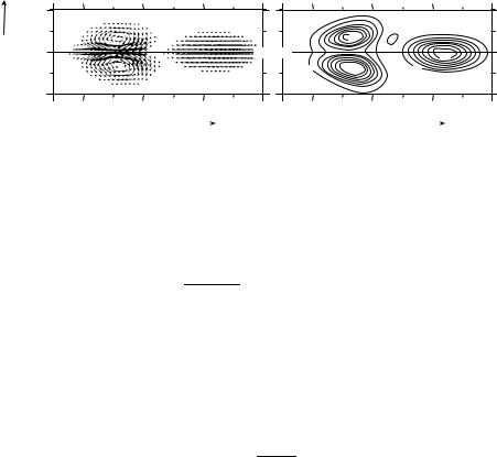


˜ |
251 |
14.5. FORECASTING EL NINO |
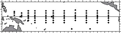
Tropical Atmosphere Ocean (TAO) Array
20 o
10 o
0 o 

-10 o |
|
|
|
|
|
|
|
|
-20 o |
|
|
|
|
Atlas |
Current Meter |
|
|
|
|
|
|
|
|
|
|
|
120 o |
140 o |
160 o |
180 o |
-160 o |
-140 o |
-120 o |
-100 o |
-80 o |
Figure 14.14 Tropical Atmosphere Ocean tao array of moored buoys operated by the noaa Pacific Marine Environmental Laboratory with help from Japan, Korea, Taiwan, and France. Figure from noaa Pacific Marine Environmental Laboratory.
The tao moorings measure air temperature, relative humidity, surface wind velocity, sea-surface temperatures, and subsurface temperatures from 10 meters down to 500 meters. Five moorings located on the equator at 110◦W, 140◦W, 170◦W, 165◦E, and 147◦E also carry upward-looking Acoustic Doppler Current Profilers adcp to measure upper-ocean currents between 10 m and 250 m. Data are sent back through the Argos system, and data are processed and made available in near real time. The moorings are recovered and replaced yearly. All sensors are calibrated prior to deployment and after recovery.
Data from tao are merged with altimeter data from Jasin, and ers-2 to obtain a more comprehensive measurement of El Ni˜no. Jasin and Topex/Poseidon data have been especially useful because they could be used to produce accurate maps of sea level every ten days. The maps provided detailed views of the development of the 1997–1998 El Ni˜no in near real time that were widely reproduced throughout the world. The observations (figure 10.6) show high sea level propagating from west to east, peaking in the eastern equatorial Pacific in November 1997. In addition, satellite data extended beyond the tao data region to include the entire tropical Pacific. This allowed oceanographers to look for extra-tropical influences on El Ni˜no.
Rain rates are measured by nasa’s Tropical Rainfall Measuring Mission which was specially designed for this purpose. It was launched on 27 November 1997, and it carries five instruments: the first spaceborne precipitation radar, a five-frequency microwave radiometer, a visible and infrared scanner, a cloud and earth radiant energy system, and a lightning imaging sensor. Working together, the instruments provide data necessary to produce monthly maps of tropical rainfall averaged over 500 km by 500 km areas with 15% accuracy. The grid is global between ±35◦ latitude. In addition, the satellite data are used to measure latent heat released to the atmosphere by rain, thus providing continuous monitoring of heating of the atmosphere in the tropics.
14.5Forecasting El Ni˜no
The importance of El Ni˜no to global weather patterns has led to many schemes for forecasting events in the equatorial Pacific. Several generations of models have been produced, but the skill of the forecasts has not always
252 CHAPTER 14. EQUATORIAL PROCESSES
increased. Models worked well for a few years, then failed. Failure was followed by improved models, and the cycle continued. Thus, the best models in 1991 failed to predict weak El Ni˜nos in 1993 and 1994 (Ji, Leetmaa, and Kousky, 1996). The best model of the mid 1990s failed to predict the onset of the strong El Ni˜no of 1997-1998 although a new model developed by the National Centers for Environmental Prediction made the best forecast of the development of the event. In general, the more sophisticated the model, the better the forecasts (Kerr, 1998).
The following recounts some of the more recent work to improve the forecasts. For simplicity, I describe the technique used by the National Centers for Environmental Prediction (Ji, Behringer, and Leetmaa, 1998). But Chen et al. (1995), Latif et al. (1993), and Barnett et al. (1993), among others, have all developed useful prediction models.
Atmospheric Models How well can we model atmospheric processes over the Pacific? To help answer the question, the World Climate Research Program’s Atmospheric Model Intercomparison Project (Gates, 1992) compared output from 30 di erent atmospheric numerical models for 1979 to 1988. The Variability in the Tropics: Synoptic to Intraseasonal Timescales subproject is especially important because it documents the ability of 15 atmospheric generalcirculation models to simulate the observed variability in the tropical atmosphere (Slingo et al. 1995). The models included several operated by government weather forecasting centers, including the model used for day-to-day forecasts by the European Center for Medium-Range Weather Forecasts.
The first results indicate that none of the models were able to duplicate all important interseasonal variability of the tropical atmosphere on timescales of 2 to 80 days. Models with weak intraseasonal activity tended to have a weak annual cycle. Most models seemed to simulate some important aspects of the interannual variability including El Ni˜no. The length of the time series was, however, too short to provide conclusive results on interannual variability.
The results of the substudy imply that numerical models of the atmospheric general circulation need to be improved if they are to be used to study tropical variability and the response of the atmosphere to changes in the tropical ocean.
Oceanic Models Our ability to understand El Ni˜no also depends on our ability to model the oceanic circulation in the equatorial Pacific. Because the models provide the initial conditions used for the forecasts, they must be able to assimilate up-to-date measurements of the Pacific along with heat fluxes and surface winds calculated from the atmospheric models. The measurements include sea-surface winds from scatterometers and moored buoys, surface temperature from the optimal-interpolation data set (see §6.6), subsurface temperatures from buoys and xbts, and sea level from altimetry and tide-gauges on islands.
Ji, Behringer, and Leetmaa (1998) at the National Centers for Environmental Prediction have modified the Geophysical Fluid Dynamics Laboratory’s Modular Ocean Model for use in the tropical Pacific (see §15.3 for more information about this model). It’s domain is the Pacific between 45◦S and 55◦N and between 120◦E and 70◦W. The zonal resolution is 1.5◦. The meridional resolution is within 10◦ of the equator, increasing smoothly to 1◦ pole-