

3.5. SEA FLOOR CHARTS AND DATA SETS |
33 |
|
h |
{ |
Reference |
|
Ellipsoid |
Geoid Undulation
|
S |
|
|
|
at |
|
|
|
ellite' |
|
|
|
|
s |
|
|
|
Or |
|
|
|
b |
|
|
|
it |
|
|
Ge |
|
|
|
oi |
|
|
|
d |
|
Sea |
|
|
|
|
|
|
|
Surface |
|
|
|
} |
|
|
|
Topography |
r |
|
|
(not to scale) |
Center of
Mass
Figure 3.13 A satellite altimeter measures the height of the satellite above the sea surface. When this is subtracted from the height r of the satellite’s orbit, the di erence is sea level relative to the center of earth. The shape of the surface is due to variations in gravity, which produce the geoid undulations, and to ocean currents which produce the oceanic topography, the departure of the sea surface from the geoid. The reference ellipsoid is the best smooth approximation to the geoid. The variations in the geoid, geoid undulations, and topography are greatly exaggerated in the figure. From Stewart (1985).
height of the sea surface relative to the center of mass of earth (figure 3.13). This gives the shape of the sea surface.
Many altimetric satellites have flown in space. All observed the marine geoid and the influence of sea-floor features on the geoid. The altimeters that produced the most useful data include Seasat (1978), geosat (1985–1988), ers–1 (1991– 1996), ers–2 (1995– ), Topex/Poseidon (1992–2006), Jason (2002–), and Envisat (2002). Topex/Poseidon and Jason were specially designed to make extremely accurate measurements of sea-surface height. They measure sea-surface height with an accuracy of ±0.05 m.
Satellite Altimeter Maps of the Sea-floor Topography Seasat, geosat, ers–
1, and ers–2 were operated in orbits with ground tracks spaced 3–10 km apart, which was su cient to map the geoid. By combining data from echo-sounders with data from geosat and ers–1 altimeter systems, Smith and Sandwell (1997) produced maps of the sea floor with horizontal resolution of 5–10 km and a global average depth accuracy of ±100 m.
3.5Sea Floor Charts and Data Sets
Almost all echo-sounder data have been digitized and combined to make seafloor charts. Data have been further processed and edited to produce digital data sets which are widely distributed in cd-rom format. These data have been supplemented with data from altimetric satellites to produce maps of the sea floor with horizontal resolution around 3 km.
The British Oceanographic Data Centre publishes the General Bathymetric Chart of the ocean (gebco) Digital Atlas on behalf of the Intergovernmental Oceanographic Commission of unesco and the International Hydrographic
34 |
CHAPTER 3. THE PHYSICAL SETTING |
60 o
30 o
0 o
-30 o
-60 o
0 o |
60 o |
120 o |
180 o |
-120 o |
-60 o |
0 o |
|
Walter H. F. Smith and David |
T. Sandwell Seafloor Topography |
Version 4.0 SIO September 26, 1996 |
|
© 1996 Walter H. F. Smith and David T. Sandwell |
|
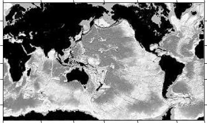
Figure 3.14 The sea-floor topography of the ocean with 3 km resolution produced from satellite altimeter observations of the shape of the sea surface. From Smith and Sandwell.
Organization. The atlas consists primarily of the location of depth contours, coastlines, and tracklines from the gebco 5th Edition published at a scale of 1:10 million. The original contours were drawn by hand based on digitized echo-sounder data plotted on base maps.
The U.S. National Geophysical Data Center publishes the etopo-2 cd-rom containing digital values of oceanic depths from echo sounders and altimetry and land heights from surveys. Data are interpolated to a 2-minute (2 nautical mile) grid. Ocean data between 64◦N and 72◦S are from the work of Smith and Sandwell (1997), who combined echo-sounder data with altimeter data from geosat and ers–1. Seafloor data northward of 64◦N are from the International Bathymetric Chart of the Arctic Ocean. Seafloor data southward of 72◦S are from are from the US Naval Oceanographic O ce’s Digital Bathymetric Data Base Variable Resolution. Land data are from the globe Project, that produced a digital elevation model with 0.5-minute (0.5 nautical mile) grid spacing using data from many nations.
National governments publish coastal and harbor maps. In the USA, the noaa National Ocean Service publishes nautical charts useful for navigation of ships in harbors and o shore waters.
3.6Sound in the Ocean
Sound provides the only convenient means for transmitting information over great distances in the ocean. Sound is used to measure the properties of the sea floor, the depth of the ocean, temperature, and currents. Whales and other ocean animals use sound to navigate, communicate over great distances, and find food.
3.6. SOUND IN THE OCEAN
|
|
|
Salinity |
|
|
|
33.0 |
33.5 |
34.0 |
34.5 |
35.0 |
|
0 |
|
|
|
|
|
-1 |
|
|
|
|
|
-2 |
|
|
|
|
( km ) |
|
|
|
|
|
Depth |
-3 |
|
|
|
|
|
|
|
|
|
|
|
-4 |
t |
|
|
S |
|
|
|
|
||
|
-5 |
|
|
|
CS |
|
|
|
|
|
|
|
-6 |
|
|
|
|
|
0 o |
5 o |
10 o |
15 o |
20 o |
|
|
|
T o C |
|
|
|
Speed Corrections ( m / s ) |
||||
0 |
20 |
40 |
60 |
80 |
100 |
|
|
Ct |
|
|
|
|
|
|
CP |
||
|
|
|
|
|
|
|
|
|
|
|
|
|
|
|
|
|
|
|
|
|
|
|
|
0 |
20 |
40 |
60 |
80 |
100 |
||||||
|
|
|
35 |
Sound Speed ( m / s ) |
|
||
1500 |
1520 |
1540 |
1560 |
|
|
|
-0 |
|
|
|
-1 |
|
|
|
-2 |
|
|
|
-3 |
|
|
|
-4 |
|
C |
|
-5 |
|
|
|
|
|
|
|
-6 |
1500 |
1520 |
1540 |
1560 |
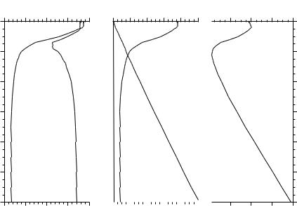
Figure 3.15 Processes producing the sound channel in the ocean. Left: Temperature T and salinity S measured as a function of depth during the R.V. Hakuho Maru cruise KH-87-1, station JT, on 28 January 1987 at Latitude 33◦52.90′ N, Long 141◦55.80′ E in the North Pacific. Center: Variations in sound speed due to variations in temperature, salinity, and depth. Right: Sound speed as a function of depth showing the velocity minimum near 1 km depth which defines the sound channel in the ocean. (Data from jpots Editorial Panel, 1991).
Sound Speed The sound speed in the ocean varies with temperature, salinity, and pressure (MacKenzie, 1981; Munk et al. 1995: 33):
C = 1448.96 + 4.591 t − 0.05304 t2 + 0.0002374 t3 + 0.0160 Z |
(3.1) |
+ (1.340 − 0.01025 t)(S − 35) + 1.675 × 10⁻⁷ Z2 − 7.139 × 10⁻¹³ t Z3
where C is speed in m/s, t is temperature in Celsius, S is salinity (see Chapter 6 for a definition of salinity), and Z is depth in meters. The equation has an accuracy of about 0.1 m/s (Dushaw et al. 1993). Other sound-speed equations have been widely used, especially an equation proposed by Wilson (1960) which has been widely used by the U.S. Navy.
For typical oceanic conditions, C is usually between 1450 m/s and 1550 m/s (figure 3.15). Using (3.1), we can calculate the sensitivity of C to changes of temperature, depth, and salinity typical of the ocean. The approximate values are: 40 m/s per 10◦C rise of temperature, 16 m/s per 1000 m increase in depth, and 1.5 m/s per 1 increase in salinity. Thus the primary causes of variability of sound speed is temperature and depth (pressure). Variations of salinity are too small to have much influence.
If we plot sound speed as a function of depth, we find that the speed usually

36 |
|
|
|
-0 |
|
|
-1 |
axis |
|
|
|
k m ) |
-2 |
|
Depth ( |
|
|
|
-3 |
|
|
-4 |
|
|
1.50 |
1.55 |
|
|
C ( k m / s ) |
CHAPTER 3. THE PHYSICAL SETTING
|
ray +8 |
|
|
+9 |
|
|
+10 |
|
|
-9 |
|
0 |
100 |
200 |
|
Range ( k m ) |
|
Figure 3.16 Ray paths of sound in the ocean for a source near the axis of the sound channel. After Munk et al. (1995).
has a minimum at a depth around 1000 m (figure 3.16). The depth of minimum speed is called the sound channel . It occurs in all ocean, and it usually reaches the surface at very high latitudes.
The sound channel is important because sound in the channel can travel very far, sometimes half way around the earth. Here is how the channel works: Sound rays that begin to travel out of the channel are refracted back toward the center of the channel. Rays propagating upward at small angles to the horizontal are bent downward, and rays propagating downward at small angles to the horizontal are bent upward (figure 3.16). Typical depths of the channel vary from 10 m to 1200 m depending on geographical area.
Absorption of Sound Absorption of sound per unit distance depends on the intensity I of the sound:
dI = −kI0 dx |
(3.2) |
where I0 is the intensity before absorption and k is an absorption coe cient which depends on frequency of the sound. The equation has the solution:
I = I0 exp(−kx) |
(3.3) |
Typical values of k (in decibels dB per kilometer) are: 0.08 dB/km at 1000 Hz, and 50 dB/km at 100,000 Hz. Decibels are calculated from: dB = 10 log(I/I0), where I0 is the original acoustic power, I is the acoustic power after absorption.
For example, at a range of 1 km a 1000 Hz signal is attenuated by only 1.8%: I = 0.982I0. At a range of 1 km a 100,000 Hz signal is reduced to I = 10−5I0. The 30,000 Hz signal used by typical echo sounders to map the ocean’s depths are little attenuated going from the surface to the bottom and back.
Very low frequency sounds in the sound channel, those with frequencies below 500 Hz have been detected at distances of megameters. In 1960 15-Hz sounds from explosions set o in the sound channel o Perth Australia were