Summary The turbulent eddy viscosities Ax, Ay , and Az cannot be calculated accurately for most oceanic flows.

1.They can be estimated from measurements of turbulent flows. Measurements in the ocean, however, are di cult. Measurements in the lab, although accurate, cannot reach Reynolds numbers of 1011 typical of the ocean.

2.The statistical theory of turbulence gives useful insight into the role of turbulence in the ocean, and this is an area of active research.

Table 8.1 Some Values for Viscosity

8.4Mixing in the Ocean

Turbulence in the ocean leads to mixing. Because the ocean has stable stratification, vertical displacement must work against the buoyancy force. Vertical mixing requires more energy than horizontal mixing. As a result, horizontal mixing along surfaces of constant density is much larger than vertical mixing across surfaces of constant density. The latter, however, usually called diapycnal mixing, is very important because it changes the vertical structure of the ocean, and it controls to a large extent the rate at which deep water eventually reaches the surface in mid and low latitudes.

The equations describing mixing depend on many processes. See Garrett (2006) for a good overview of the subject. Here I consider some simple flows. A simple equation for vertical mixing by eddies of a tracer Θ such as salt or temperature is:

where Az is the vertical eddy di usivity, W is a mean vertical velocity, and S is a source term.

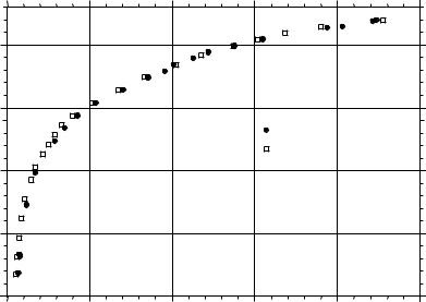
Average Vertical Mixing Walter Munk (1966) used a very simple observation to calculate vertical mixing in the ocean. He observed that the ocean has a thermocline almost everywhere, and the deeper part of the thermocline does not change even over decades (figure 8.4). This was a remarkable observation because we expect downward mixing would continuously deepen the thermocline. But it doesn’t. Therefore, a steady-state thermocline requires that the downward mixing of heat by turbulence must be balanced by an upward transport of heat by a mean vertical current W . This follows from (8.21) for steady

Measured Vertical Mixing Direct observations of vertical mixing required the development of techniques for measuring: i) the fine structure of turbulence, including probes able to measure temperature and salinity with a spatial resolution of a few centimeters (Gregg 1991), and ii) the distribution of tracers such as sulphur hexafluoride (SF6) which can be easily detected at concentrations as small as one gram in a cubic kilometer of seawater.

Direct measurements of open-ocean turbulence and the di usion of SF6 yield an eddy di usivity:

Az ≈ 1 × 10−5 m2/s Open-Ocean Vertical Eddy Di usivity (8.25)

For example, Ledwell, Watson, and Law (1998) injected 139 kg of SF6 in the Atlantic near 26◦N, 29◦W 1200 km west of the Canary Islands at a depth of 310 m. They then measured the concentration for five months as it mixed over hundreds of kilometers to obtain a diapycnal eddy di usivity of Az = 1.2 ± 0.2 × 10−5 m2/s.

The large discrepancy between Munk’s calculation of the average eddy diffusivity for vertical mixing and the small values observed in the open ocean has

Polzin et al. (1997) measured the vertical structure of temperature in the Brazil Basin in the south Atlantic. They found Az > 10−3 m2/s close to the bottom when the water flowed over the western flank of the mid-Atlantic ridge at the eastern edge of the basin. Kunze and Toole (1997) calculated enhanced eddy di usivity as large as A = 10−3 m2/s above Fieberling Guyot in the Northwest Pacific and smaller di usivity along the flank of the seamount. And, Garbato et al (2004) calculated even stronger mixing in the Scotia Sea where the Antarctic Circumpolar Current flows between Antarctica and South America.

The results of these and other experiments show that mixing occurs mostly by breaking internal waves and by shear at oceanic boundaries: along continental slopes, above seamounts and mid-ocean ridges, at fronts, and in the mixed layer at the sea surface. To a large extent, the mixing is driven by deep-ocean tidal currents, which become turbulent when they flow past obstacles on the sea floor, including seamounts and mid-ocean ridges (Jayne et al, 2004).

Because water is mixed along boundaries or in other regions (Gnadadesikan, 1999), we must take care in interpreting temperature profiles such as that in figure 8.4. For example, water at 1200 m in the central north Atlantic could move horizontally to the Gulf Stream, where it mixes with water from 1000 m. The mixed water may then move horizontally back into the central north Atlantic at a depth of 1100 m. Thus parcels of water at 1200 m and at 1100 m at some location may reach their position along entirely di erent paths.

Measured Horizontal Mixing Eddies mix fluid in the horizontal, and large eddies mix more fluid than small eddies. Eddies range in size from a few meters due to turbulence in the thermocline up to several hundred kilometers for geostrophic eddies discussed in Chapter 10.

In general, mixing depends on Reynolds number R (Tennekes 1990: p. 11)

where γ is the molecular di usivity of heat, U is a typical velocity in an eddy, and L is the typical size of an eddy. Furthermore, horizontal eddy di usivity are ten thousand to ten million times larger than the average vertical eddy di usivity.

Equation (8.27) implies Ax U L. This functional form agrees well with Joseph and Sender’s (1958) analysis, as reported in (Bowden 1962) of spreading of radioactive tracers, optical turbidity, and Mediterranean Sea water in the north Atlantic. They report

10 km < L < 1500 km

P = 0.01 ± 0.005 m/s

where L is the distance from the source, and P is a constant.

The horizontal eddy di usivity (8.28) also agrees well with more recent reports of horizontal di usivity. Work by Holloway (1986) who used satellite altimeter observations of geostrophic currents, Freeland who tracked sofar underwater floats, and Ledwell Watson, and Law (1998) who used observations of

Using (8.28) and the measured Ax implies eddies with typical scales of 80 km, a value near the size of geostrophic eddies responsible for the mixing.

Ledwell, Watson, and Law (1998) also measured a horizontal eddy di usivity. They found

over scales of meters due to turbulence in the thermocline probably driven by breaking internal waves. This value, when used in (8.28) implies typical lengths of 100 m for the small eddies responsible for mixing in this experiment.

Comments on horizontal mixing

1.Horizontal eddy di usivity is 105 − 108 times larger than vertical eddy di usivity.

2.Water in the interior of the ocean moves along sloping surfaces of constant density with little local mixing until it reaches a boundary where it is mixed vertically. The mixed water then moves back into the open ocean again along surfaces of constant density (Gregg 1987).

One particular case is particularly noteworthy. When water, mixing downward through the base of the mixed layer, flows out into the thermocline along surfaces of constant density, the mixing leads to the ventilated thermocline model of oceanic density distributions.