coasts of the United States (Graber et al, 2006). The model uses a finite-element grid, the Boussinesq approximation, quadratic bottom friction, and vertically integrated continuity and momentum equations for flow on a rotating earth. It can be run as either a two-dimensional, depth-integrated model, or as a three-dimensional model. Because waves contribute to storm surges, the model includes waves calculated from the wam third-geneation wave model (see §16.5).

The model is forced by:

1.High resolution winds and surface pressure obtained by combining weather forecasts from the noaa National Weather Service and the National Hurricane Center along the o cial and alternate forecast storm tracks.

2.Tides at the open-ocean boundaries of the model.

3.Sea-surface height and currents at the open-ocean boundaries of the model.

The model successfully forecast the Hurricane Katrina storm surge, giving values in excess of 6.1 m near New Orleans.

15.5Assimilation Models

Many of the models I have described so far have output, such as current velocity or surface topography, constrained by oceanic observations of the variables they calculate. Such models are called assimilation models. In this section, I will consider how data can be assimilated into numerical models.

Let’s begin with a primitive-equation, eddy-admitting numerical model used to calculate the position of the Gulf Stream. Let’s assume that the model is driven with real-time surface winds from the ecmwf weather model. Using the model, we can calculate the position of the current and also the sea-surface topography associated with the current. We find that the position of the Gulf Stream wiggles o shore of Cape Hatteras due to instabilities, and the position calculated by the model is just one of many possible positions for the same wind forcing. Which position is correct, that is, what is the position of the current today? We know, from satellite altimetry, the position of the current at a few points a few days ago. Can we use this information to calculate the current’s position today? How do we assimilate this information into the model?

Many di erent approaches are being explored (Malanotte-Rizzoli, 1996). Roger Daley (1991) gives a complete description of how data are used with atmospheric models. Andrew Bennet (1992) and Carl Wunsch (1996) describe oceanic applications.

The di erent approaches are necessary because assimilation of data into models is not easy.

1.Data assimilation is an inverse problem: A finite number of observations are used to estimate a continuous field—a function, which has an infinite number of points. The calculated fields, the solution to the inverse problem, are completely under-determined. There are many fields that fit the observations and the model precisely, and the solutions are not unique. In our example, the position of the Gulf Stream is a function. We may not need an infinite number of values to specify the position of the stream if

we assume the position is somewhat smooth in space. But we certainly need hundreds of values along the stream’s axis. Yet, we have only a few satellite points to constrain the position of the Stream.

To learn more about inverse problems and their solution, read Parker (1994) who gives a very good introduction based on geophysical examples.

2.Ocean dynamics are non-linear, while most methods for calculating solutions to inverse problems depend on linear approximations. For example the position of the Gulf Stream is a very nonlinear function of the forcing by wind and heat fluxes over the north Atlantic.

3.Both the model and the data are incomplete and both have errors. For example, we have altimeter measurements only along the tracks such as those shown in figure 2.6, and the measurements have errors of ±2 cm.

4.Most data available for assimilation into data comes from the surface, such as avhrr and altimeter data. Surface data obviously constrain the surface geostrophic velocity, and surface velocity is related to deeper velocities. The trick is to couple the surface observations to deeper currents.

While various techniques are used to constrain numerical models in oceanography, perhaps the most practical are techniques borrowed from meteorology.

Most major ocean currents have dynamics which are significantly nonlinear. This precludes the ready development of inverse methods. . . Accordingly, most attempts to combine ocean models and measurements have followed the practice in operational meteorology: measurements are used to prepare initial conditions for the model, which is then integrated forward in time until further measurements are available. The model is thereupon re-initialized. Such a strategy may be described as sequential.—Bennet (1992).

Let’s see how Professor Allan Robinson and colleagues at Harvard University used sequential estimation techniques to make the first forecasts of the Gulf Stream using a very simple model.

The Harvard Open-Ocean Model was an eddy-admitting, quasi-geostropic model of the Gulf Stream east of Cape Hatteras (Robinson et al. 1989). It had six levels in the vertical, 15 km resolution, and one-hour time steps. It used a filter to smooth high-frequency variability and to damp grid-scale variability.

By quasi-geostrophic we mean that the flow field is close to geostrophic balance. The equations of motion include the acceleration terms D/Dt, where D/Dt is the substantial derivative and t is time. The flow can be stratified, but there is no change in density due to heat fluxes or vertical mixing. Thus the quasi-geostrophic equations are simpler than the primitive equations, and they could be integrated much faster. Cushman-Roisin (1994: 204) gives a good description of the development of quasi-geostrophic equations of motion.

The model reproduces the important features of the Gulf Stream and it’s extension, including meanders, coldand warm-core rings, the interaction of rings with the stream, and baroclinic instability (figure 15.4). Because the

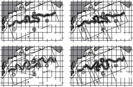
Figure 15.4 Output from the Harvard Open-Ocean Model: A the initial state of the model, the analysis, and B Data used to produce the analysis for 2 March 1988. C The forecast for 9 March 1988. D The analysis for 9 March. Although the Gulf Stream changed substantially in one week, the model forecasts the changes well. After Robinson et al. (1989).

model was designed to forecast the dynamics of the Gulf Stream, it must be constrained by oceanic measurements:

1.Data provide the initial conditions for the model. Satellite measurements of sea-surface temperature from the avhrr and topography from an altimeter are used to determine the location of features in the region. Expendable bathythermograph, axbt measurements of subsurface temperature, and historical measurements of internal density are also used. The features are represented by an analytic functions in the model.

2.The data are introduced into the numerical model, which interpolates and smoothes the data to produce the best estimate of the initial fields of density and velocity. The resulting fields are called an analysis.

3.The model is integrated forward for one week, when new data are available, to produce a forecast.

4.Finally, the new data are introduced into the model as in the first step above, and the processes is repeated.

The model made useful, one-week forecasts of the Gulf Stream region. Much more advanced models with much higher resolution are now being used to make global forecasts of ocean currents up to one month in advance in support of the Global Ocean Data Assimilation Experiment godae that started in 2003. The goal of godae is produce routine oceanic forecasts similar to todays weather forecasts.

An example of a godae model is the global US Navy Layered Ocean Model. It is a primitive equation model with 1/32◦ resolution in the horizontal and seven layers in the vertical. It assimilates altimeter data from Jason, Geosat Follow-on (gfo), and ers-2 satellites and sea-surface temperature from avhrr on noaa satellites. The model is forced with winds and heat fluxes for up to five days in the future using output from the Navy Operational Global Atmospheric Prediction System. Beyond five days, seasonal mean winds and fluxes are used. The model is run daily (figure 15.5) and produces forecasts for up to one month in the future. The model has useful skill out to about 20 days.

1/16° Global Navy Layed Ocean Model Sea-Surface Height and Current

45°N

40°N

35°N

30°N

Analysis for 25 June 2003

Sea-Surface Height (cm)

Figure 15.5 Analysis of the Gulf Stream region from the Navy Layered Ocean Model. From the U.S. Naval Oceanographic O ce.

A group of French laboratories and agencies operates a similar operational forecasting system, Mercator, based on assimilation of altimeter measurements of sea-surface height, satellite measurements of sea-surface temperature, and internal density fields in the ocean, and currents at 1000 m from thousands of Argo floats. Their model has 1/15◦ resolution in the Atlantic and 2◦ globally.

15.6Coupled Ocean and Atmosphere Models

Coupled numerical models of the atmosphere and ocean are used to study the climate, its variability, and its response to external forcing. The most important use of the models has been to study how earth’s climate might respond to a doubling of CO2 in the atmosphere. Much of the literature on climate change is based on studies using such models. Other important uses of coupled models include studies of El Ni˜no and the meridional overturning circulation. The former varies over a few years, the latter varies over a few centuries.

Development of the coupled models tends to be coordinated through the World Climate Research Program of the World Meteorological Organization

wcrp/wmo, and recent progress is summarized in Chapter 8 of the Climate Change 2001: The Scientific Basis report by the Intergovernmental Panel on Climate Change (ipcc, 2007).

Many coupled ocean and atmosphere models have been developed. Some include only physical processes in the ocean, atmosphere, and the ice-covered polar seas. Others add the influence of land and biological activity in the ocean. Let’s look at the oceanic components of a few models.

Climate System Model The Climate System Model developed by the National Center for Atmospheric Research ncar includes physical and biogeochemical influence on the climate system (Boville and Gent, 1998). It has atmosphere, ocean, land-surface, and sea-ice components coupled by fluxes between components. The atmospheric component is the ncar Community Climate Model, the oceanic component is a modified version of the Princeton Modular Ocean Model, using the Gent and McWilliams (1990) scheme for parameterizing mesoscale eddies. Resolution is approximately 2◦ × 2◦ with 45 vertical levels in the ocean.

The model has been spun up and integrated for 300 years, the results are realistic, and there is no need for a flux adjustment. (See the special issue of

Journal of Climate, June 1998).

Princeton Coupled Model The model consists of an atmospheric model with a horizontal resolution of 7.5◦ longitude by 4.5◦ latitude and 9 levels in the vertical, an ocean model with a horizontal resolution of 4◦ and 12 levels in the vertical, and a land-surface model. The ocean and atmosphere are coupled through heat, water, and momentum fluxes. Land and ocean are coupled through river runo . And land and atmosphere are coupled through water and heat fluxes.

Hadley Center Model This is an atmosphere-ocean-ice model that minimizes the need for flux adjustments (Johns et al, 1997). The ocean component is based on the Bryan-Cox primitive equation model, with realistic bottom features, vertical mixing coe cients from Pacanowski and Philander (1981). Both the ocean and the atmospheric component have a horizontal resolution of 96 × 73 grid points, the ocean has 20 levels in the vertical.

In contrast to most coupled models, this one is spun up as a coupled system with flux adjustments during spin up to keep sea surface temperature and salinity close to observed mean values. The coupled model was integrated from rest using Levitus values for temperature and salinity for September. The initial integration was from 1850 to 1940. The model was then integrated for another 1000 years. No flux adjustment was necessary after the initial 140-year integration because drift of global-averaged air temperature was ≤ 0.016 K/century.

Comments on Accuracy of Coupled Models Models of the coupled, land- air-ice-ocean climate system must simulate hundreds to thousands of years. Yet,

It will be very hard to establish an integration framework, particularly on a global scale, as present capabilities for modelling the earth system are rather limited. A dual approach is planned. On the one hand, the relatively conventional approach of improving coupled atmosphere-ocean- land-ice models will be pursued. Ingenuity aside, the computational de-

mands are extreme, as is borne out by the Earth System Simulator — 640 linked supercomputers providing 40 teraflops [1012 floating-point operations per second] and a cooling system from hell under one roof — to be built in Japan by 2003.— Newton, 1999.

Because models must be simplified to run on existing computers, the models must be simpler than models that simulate flow for a few years (wcrp, 1995).

In addition, the coupled model must be integrated for many years for the ocean and atmosphere to approach equilibrium. As the integration proceeds, the coupled system tends to drift away from reality due to errors in calculating fluxes of heat and momentum between the ocean and atmosphere. For example, very small errors in precipitation over the Antarctic Circumpolar Current leads to small changes the salinity of the current, which leads to large changes in deep convection in the Weddell Sea, which greatly influences the volume of deep water masses.

Some modelers allow the system to drift, others adjust sea-surface temperature and the calculated fluxes between the ocean and atmosphere. Returning to the example, the flux of fresh water in the circumpolar current could be adjusted to keep salinity close to the observed value in the current. There is no good scientific basis for the adjustments except the desire to produce a “good” coupled model. Hence, the adjustments are ad hoc and controversial. Such adjustments are called flux adjustments or flux corrections.

Fortunately, as models have improved, the need for adjustment or the magnitude of the adjustment has been reduced. For example, using the GentMcWilliams scheme for mixing along constant-density surfaces in a coupled ocean-atmosphere model greatly reduced climate drift in a coupled ocean-atmos- phere model because the mixing scheme reduced deep convection in the Antarctic Circumpolar Current and elsewhere (Hirst, O’Farrell, and Gordon, 2000).

Grassl (2000) lists four capabilities of a credible coupled general circulation model:

1.“Adequate representation of the present climate.

2.“Reproduction (within typical interannual and decades time-scale climate variability) of the changes since the start of the instrumental record for a given history of external forcing;

3.“Reproduction of a di erent climate episode in the past as derived from paleoclimate records for given estimates of the history of external forcing; and

4.“Successful simulation of the gross features of an abrupt climate change event from the past.”

McAvaney et al. (2001) compared the oceanic component of twenty-four coupled models, including models with and without flux adjustments. They found substantial di erences among the models. For example, only five models calculated a meridional overturning circulation within 10% the observed value of 20 Sv. Some had values as low as 3 Sv, others had values as large as 36 Sv. Most