8.2Turbulence

Dye

Glass Tube

Valve

Water

Figure 8.2 Reynolds apparatus for investigating the transition to turbulence in pipe flow, with photographs of near-laminar flow (left) and turbulent flow (right) in a clear pipe much like the one used by Reynolds. After Binder (1949: 88-89).

where, U is a typical velocity of the flow and L is a typical length describing the flow. You are free to pick whatever U, L might be typical of the flow. For example L can be either a typical cross-stream distance, or an along-stream distance. Typical values in the open ocean are U = 0.1 m/s and L = 1 megameter, so Re = 1011. Because non-linear terms are important if Re > 10 – 1000, they are certainly important in the ocean. The ocean is turbulent.

The Reynolds number is named after Osborne Reynolds (1842–1912) who conducted experiments in the late 19th century to understand turbulence. In one famous experiment (Reynolds 1883), he injected dye into water flowing at various speeds through a tube (figure 8.2). If the speed was small, the flow was smooth. This is called laminar flow. At higher speeds, the flow became irregular and turbulent. The transition occurred at Re = V D/ν ≈ 2000, where V is the average speed in the pipe, and D is the diameter of the pipe.

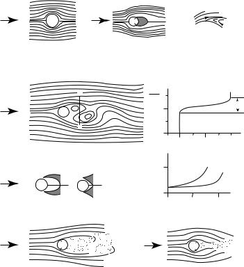
As Reynolds number increases above some critical value, the flow becomes more and more turbulent. Note that flow pattern is a function of Reynold’s number. All flows with the same geometry and the same Reynolds number have the same flow pattern. Thus flow around all circular cylinders, whether 1 mm or 1 m in diameter, look the same as the flow at the top of figure 8.3 if the Reynolds number is 20. Furthermore, the boundary layer is confined to a very thin layer close to the cylinder, in a layer too thin to show in the figure.

Turbulent Stresses: The Reynolds Stress Prandtl, Karman and others who studied fluid mechanics in the early 20th century, hypothesized that parcels of fluid in a turbulent flow played the same role in transferring momentum within the flow that molecules played in laminar flow. The work led to the idea of turbulent stresses.

To see how these stresses might arise, consider the momentum equation for

Figure 8.3 Flow past a circular cylinder as a function of Reynolds number between one and a million. From Richardson (1961). The appropriate flows are: A—a toothpick moving at 1 mm/s; B—finger moving at 2 cm/s; F—hand out a car window at 60 mph. All flow at the same Reynolds number has the same streamlines. Flow past a 10 cm diameter cylinder at 1 cm/s looks the same as 10 cm/s flow past a cylinder 1 cm in diameter because in both cases Re = 1000.

The second equation follows from the first since hU ∂u′/∂xi = 0 and hu′ ∂U/∂xi

=0, which follow from the definition of U : hU ∂u′/∂xi = U ∂hu′i/∂x = 0. Using (8.5) in (7.19) gives:

Subtracting the mean of (8.8) from (8.8) splits the continuity equation into two equations:

Using (8.5) in (8.1) taking the mean value of the resulting equation, then simplifying using (8.7), the x-component of the momentum equation for the mean flow becomes:

(8.10)

The derivation is not as simple as it seems. See Hinze (1975: 22) for details. Thus the additional force per unit mass due to the turbulence is:

The terms ρhu′u′i, ρhu′v′i, and ρhu′w′i transfer eastward momentum (ρu′) in the x, y, and z directions. For example, the term ρhu′w′i gives the downward transport of eastward momentum across a horizontal plane. Because they transfer momentum, and because they were first derived by Osborne Reynolds, they are called Reynolds Stresses.

8.3Calculation of Reynolds Stress:

The Reynolds stresses such as ∂hu′w′i/∂z are called virtual stresses (cf. Goldstein, 1965: §69 & §81) because we assume that they play the same role as the viscous terms in the equation of motion. To proceed further, we need values or functional form for the Reynolds stress. Several approaches are used.

From Experiments We can calculate Reynolds stresses from direct measurements of (u′, v′, w′) made in the laboratory or ocean. This is accurate, but hard to generalize to other flows. So we seek more general approaches.

By Analogy with Molecular Viscosity Let’s return to the example in figure 8.1, which shows flow above a surface in the x, y plane. Prandtl, in a revolutionary paper published in 1904, stated that turbulent viscous e ects are only important in a very thin layer close to the surface, the boundary layer. Prandtl’s invention of the boundary layer allows us to describe very accurately turbulent flow of wind above the sea surface, or flow at the bottom boundary layer in the ocean, or flow in the mixed layer at the sea surface. See the box

Turbulent Boundary Layer Over a Flat Plate.

To calculate flow in a boundary layer, we assume that flow is constant in the x, y direction, that the statistical properties of the flow vary only in the z direction, and that the mean flow is steady. Therefore ∂/∂t = ∂/∂x = ∂/∂y = 0, and (8.10) can be written:

We now assume, in analogy with (8.2)

where Az is an eddy viscosity or eddy di usivity which replaces the molecular viscosity ν in (8.2). With this assumption,

where I have assumed that Az is either constant or that it varies more slowly in the z direction than ∂U/∂z. Later, I will assume that Az ≈ z.

Because eddies can mix heat, salt, or other properties as well as momentum, I will use the term eddy di usivity. It is more general than eddy viscosity, which is the mixing of momentum.

The x and y momentum equations for a homogeneous, steady-state, turbulent boundary layer above or below a horizontal surface are:

where f = 2ω sin ϕ is the Coriolis parameter, and I have dropped the molecular viscosity term because it is much smaller than the turbulent eddy viscosity. Note, (8.15b) follows from a similar derivation from the y-component of the momentum equation. We will need (8.15) when we describe flow near the surface.

The assumption that an eddy viscosity Az can be used to relate the Reynolds stress to the mean flow works well in turbulent boundary layers. However Az cannot be obtained from theory. It must be calculated from data collected in wind tunnels or measured in the surface boundary layer at sea. See Hinze (1975,

Prandtl’s theory based on assumption (8.13) works well only where friction is much larger than the Coriolis force. This is true for air flow within tens of meters of the sea surface and for water flow within a few meters of the surface. The application of the technique to other flows in the ocean is less clear. For example, the flow in the mixed layer at depths below about ten meters is less well described by the classical turbulent theory. Tennekes and Lumley (1990: 57) write:

Mixing-length and eddy viscosity models should be used only to generate analytical expressions for the Reynolds stress and mean-velocity profile if those are desired for curve fitting purposes in turbulent flows characterized by a single length scale and a single velocity scale. The use of mixing-length theory in turbulent flows whose scaling laws are not known beforehand should be avoided.

Problems with the eddy-viscosity approach:

1.Except in boundary layers a few meters thick, geophysical flows may be influenced by several characteristic scales. For example, in the atmospheric boundary layer above the sea, at least three scales may be important: i) the height above the sea z, ii) the Monin-Obukhov scale L discussed in §4.3, and iii) the typical velocity U divided by the Coriolis parameter U/f .

2.The velocities u′, w′ are a property of the fluid, while Az is a property of the flow ;

3.Eddy viscosity terms are not symmetric:

hu′v′i = hv′u′i ; but

From a Statistical Theory of Turbulence The Reynolds stresses can be calculated from various theories which relate hu′u′i to higher order correlations of the form hu′u′u′i. The problem then becomes: How to calculate the higher order terms? This is the closure problem in turbulence. There is no general solution, but the approach leads to useful understanding of some forms of turbulence such as isotropic turbulence downstream of a grid in a wind tunnel (Batchelor 1967). Isotropic turbulence is turbulence with statistical properties that are independent of direction.

The approach can be modified somewhat for flow in the ocean. In the idealized case of high Reynolds flow, we can calculate the statistical properties of a flow in thermodynamic equilibrium. Because the actual flow in the ocean is far from equilibrium, we assume it will evolve towards equilibrium. Holloway (1986) provides a good review of this approach, showing how it can be used to derive the influence of turbulence on mixing and heat transports. One interesting result of the work is that zonal mixing ought to be larger than meridional mixing.