Latitude (degrees)

Figure 9.6 Angle between the wind and flow at the surface calculated by Maximenko and Niiler using positions from drifters drogued at 15 m with satellite-altimeter, gravity, and grace data and winds from the ncar/ncep reanalysis.

falls below the critical value (Pollard et al. 1973). This idea, when included in p

mixed-layer theories, leads to a surface current V0 that is proportional to N/f

Notice that (9.22) and (9.23) are now dimensionally correct. The equations used earlier, (9.14), (9.16), (9.20), and (9.21) all required a dimensional coe cient.

9.3Ekman Mass Transport

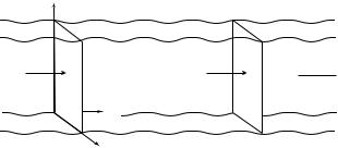
Flow in the Ekman layer at the sea surface carries mass. For many reasons we may want to know the total mass transported in the layer. The Ekman mass transport ME is defined as the integral of the Ekman velocity UE , VE from the surface to a depth d below the Ekman layer. The two components of the transport are MEx, MEy :

The transport has units kg/(m·s). It is the mass of water passing through a vertical plane one meter wide that is perpendicular to the transport and extending from the surface to depth −d (figure 9.7).

We calculate the Ekman mass transports by integrating (8.15) in (9.24):

measured winds using (9.26) and (9.27), and Qy = 13.5 ± 0.3 Sv from mean winds averaged over many years at 11◦N.

Use of Transports Mass transports are widely used for two important reasons. First, the calculation is much more robust than calculations of velocities in the Ekman layer. By robust, I mean that the calculation is based on fewer assumptions, and that the results are more likely to be correct. Thus the calculated mass transport does not depend on knowing the distribution of velocity in the Ekman layer or the eddy viscosity.

Second, the variability of transport in space has important consequences. Let’s look at a few applications.

9.4Application of Ekman Theory

Because steady winds blowing on the sea surface produce an Ekman layer that transports water at right angles to the wind direction, any spatial variability of the wind, or winds blowing along some coasts, can lead to upwelling. And upwelling is important:

1.Upwelling enhances biological productivity, which feeds fisheries.

2.Cold upwelled water alters local weather. Weather onshore of regions of upwelling tend to have fog, low stratus clouds, a stable stratified atmosphere, little convection, and little rain.

3.Spatial variability of transports in the open ocean leads to upwelling and downwelling, which leads to redistribution of mass in the ocean, which leads to wind-driven geostrophic currents via Ekman pumping.

Coastal Upwelling To see how winds lead to upwelling, consider north winds blowing parallel to the California Coast (figure 9.8 left). The winds produce a mass transport away from the shore everywhere along the shore. The water pushed o shore can be replaced only by water from below the Ekman layer. This is upwelling (figure 9.8 right). Because the upwelled water is cold, the upwelling leads to a region of cold water at the surface along the coast. Figure 10.16 shows the distribution of cold water o the coast of California.

Upwelled water is colder than water normally found on the surface, and it is richer in nutrients. The nutrients fertilize phytoplankton in the mixed layer, which are eaten by zooplankton, which are eaten by small fish, which are eaten by larger fish and so on to infinity. As a result, upwelling regions are productive waters supporting the world’s major fisheries. The important regions are o shore of Peru, California, Somalia, Morocco, and Namibia.

Now I can answer the question I asked at the beginning of the chapter: Why is the climate of San Francisco so di erent from that of Norfolk, Virginia? Figures 4.2 or 9.8 show that wind along the California and Oregon coasts has a strong southward component. The wind causes upwelling along the coast, which leads to cold water close to shore. The shoreward component of the wind brings warmer air from far o shore over the colder water, which cools the incoming air close to the sea, leading to a thin, cool atmospheric boundary layer. As the air cools, fog forms along the coast. Finally, the cool layer of air is blown over