

8.5. STABILITY |
127 |
3.Observations of mixing in the ocean imply that numerical models of the oceanic circulation should use mixing schemes that have di erent eddy di usivity parallel and perpendicular to surfaces of constant density, not parallel and perpendicular to level surfaces of constant z as I used above. Horizontal mixing along surfaces of constant z leads to mixing across layers of constant density because layers of constant density are inclined to the horizontal by about 10−3 radians (see §10.7 and figure 10.13).
Studies by Danabasoglu, McWilliams, and Gent (1994) show that numerical models using isopycnal and diapycnal mixing leads to much more realistic simulations of the oceanic circulation.
4.Mixing is horizontal and two dimensional for horizontal scales greater than N H/(2f ) where H is the water depth, N is the stability frequency (8.36), and f is the Coriolis parameter (Dritschel, Juarez, and Ambaum (1999).
8.5Stability
We saw in section 8.2 that fluid flow with a su ciently large Reynolds number is turbulent. This is one form of instability. Many other types of instability occur in the in the ocean. Here, let’s consider three of the more important ones: i) static stability associated with change of density with depth, ii) dynamic stability associated with velocity shear, and iii) double-di usion associated with salinity and temperature gradients in the ocean.
Static Stability and the Stability Frequency Consider first static stability. If more dense water lies above less dense water, the fluid is unstable. The more dense water will sink beneath the less dense. Conversely, if less dense water lies above more dense water, the interface between the two is stable. But how stable? We might guess that the larger the density contrast across the interface, the more stable the interface. This is an example of static stability. Static stability is important in any stratified flow where density increases with depth, and we need some criterion for determining the importance of the stability.
Consider a parcel of water that is displaced vertically and adiabatically in a stratified fluid (figure 8.5). The buoyancy force F acting on the displaced parcel is the di erence between its weight V gρ′ and the weight of the surrounding water V gρ2, where V is the volume of the parcel:
F = V g (ρ2 − ρ′)
Displaced Volume of Water V @ ρ2
Displacement Distance δz
Parcel with Density ρ'
Figure 8.5 Sketch for calculating static stability and stability frequency.

128 |
CHAPTER 8. EQUATIONS OF MOTION WITH VISCOSITY |
The acceleration of the displaced parcel is:
a = |
F |
|
= |
|
g (ρ2 − ρ′) |
|
(8.31) |
||
m |
|
||||||||
|
|
|
|
|
ρ′ |
|
|||
but |
|
|
|
|
|
|
|
|
|
ρ2 |
= ρ + |
dρ |
water δz |
(8.32) |
|||||
|
|||||||||
dz |
|||||||||
ρ′ |
= ρ + |
dρ |
parcel δz |
(8.33) |
|||||
|
|||||||||
dz |
|||||||||
Using (8.32) and (8.33) in (8.31), ignoring terms proportional to δz2, we obtain:
|
1 |
|
|
|
|
|
|
|
|
|
E = − |
ρ |
" |
|
dz water |
− |
|
dz |
parcel# |
(8.34) |
|
where E ≡ −a/(g δz) is the stability of the water column (McDougall, 1987; Sverdrup, Johnson, and Fleming, 1942: 416; or Gill, 1982: 50).
In the upper kilometer of the ocean stability is large, and the first term in (8.34) is much larger than the second. The first term is proportional to the rate of change of density of the water column. The second term is proportional to the compressibility of sea water, which is very small. Neglecting the second term, we can write the stability equation:
E ≈ − |
1 dρ |
(8.35) |
ρ dz |
The approximation used to derive (8.35) is valid for E > 50 × 10−8/m.
Below about a kilometer in the ocean, the change in density with depth is so small that we must consider the small change in density of the parcel due to changes in pressure as it is moved vertically.
Stability is defined such that
E > 0 Stable
E = 0 Neutral Stability
E < 0 Unstable
In the upper kilometer of the ocean, z < 1, 000 m, E = (50—1000) × 10−8/m, and in deep trenches where z > 7, 000 m, E = 1 × 10⁻⁸/m.
The influence of stability is usually expressed by a stability frequency N :
N 2 ≡ −gE |
(8.36) |
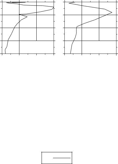
The stability frequency is often called the buoyancy frequency or the BruntVaisala frequency. The frequency quantifies the importance of stability, and it is a fundamental variable in the dynamics of stratified flow. In simplest terms, the frequency can be interpreted as the vertical frequency excited by a vertical displacement of a fluid parcel. Thus, it is the maximum frequency of internal waves in the ocean. Typical values of N are a few cycles per hour (figure 8.6).
8.5. STABILITY |
129 |
|
0 |
|
|
|
|
|
|
-0 |
(decibars)Depth |
1000 |
|
|
|
|
|
|
-100 |
2000 |
|
|
|
|
|
|
-200 |
|
|
|
|
|
|
|
|
||
|
3000 |
|
|
|
|
|
|
-300 |
|
|
|
35.0 ° N, 151.9 ° E |
|
|
|
7.5 ° N, 137.0 ° E |
|
|
|
|
24 April 1976 |
|
|
|
16 June 1974 |
|
|
4000 |
|
|
|
|
|
|
-400 |
|
0 |
1 |
2 |
3 |
0 |
5 |
10 |
15 |
|
|
|
Stability Frequency (cycles per hour) |
|
|
|||
Figure 8.6. Observed stability frequency in the Pacific. Left: Stability of the deep thermocline east of the Kuroshio. Right: Stability of a shallow thermocline typical of the tropics. Note the change of scales.
Dynamic Stability and Richardson’s Number If velocity changes with depth in a stable, stratified flow, then the flow may become unstable if the change in velocity with depth, the current shear , is large enough. The simplest example is wind blowing over the ocean. In this case, stability is very large across the sea surface. We might say it is infinite because there is a step discontinuity in ρ, and (8.36) is infinite. Yet, wind blowing on the ocean creates waves, and if the wind is strong enough, the surface becomes unstable and the waves break.
This is an example of dynamic instability in which a stable fluid is made unstable by velocity shear. Another example of dynamic instability, the KelvinHelmholtz instability, occurs when the density contrast in a sheared flow is much less than at the sea surface, such as in the thermocline or at the top of a stable, atmospheric boundary layer (figure 8.7).
The relative importance of static stability and dynamic instability is expressed by the Richardson Number :
Ri ≡ |
g E |
(8.37) |
(∂U/∂z)2 |
where the numerator is the strength of the static stability, and the denominator is the strength of the velocity shear.
Ri > 0.25 Stable
Ri < 0.25 Velocity Shear Enhances Turbulence
Note that a small Richardson number is not the only criterion for instability. The Reynolds number must be large and the Richardson number must be less than 0.25 for turbulence. These criteria are met in some oceanic flows. The turbulence mixes fluid in the vertical, leading to a vertical eddy viscosity and eddy di usivity. Because the ocean tends to be strongly stratified and currents tend to be weak, turbulent mixing is intermittent and rare. Measurements of

130 |
CHAPTER 8. EQUATIONS OF MOTION WITH VISCOSITY |
Figure 8.7 Billow clouds showing a Kelvin-Helmholtz instability at the top of a stable atmospheric layer. Some billows can become large enough that more dense air overlies less dense air, and then the billows collapse into turbulence. Photography copyright Brooks Martner, noaa Environmental Technology Laboratory.
density as a function of depth rarely show more dense fluid over less dense fluid as seen in the breaking waves in figure 8.7 (Moum and Caldwell 1985).
Double Di usion and Salt Fingers In some regions of the ocean, less dense water overlies more dense water, yet the water column is unstable even if there are no currents. The instability occurs because the molecular di usion of heat is about 100 times faster than the molecular di usion of salt. The instability was first discovered by Melvin Stern in 1960 who quickly realized its importance in oceanography.
Initial Density |
Density after a few minutes |
Warm, Salty ρ1
Warm, Salty ρ1
Cold, Salty ρ > ρ2
Cold, Less Salty ρ2
Cold, Less Salty ρ2
Figure 8.8 Left: Initial distribution of density in the vertical. Right: After some time, the di usion of heat leads to a thin unstable layer between the two initially stable layers. The thin unstable layer sinks into the lower layer as salty fingers. The vertical scale in the figures is a few centimeters.
Consider two thin layers a few meters thick separated by a sharp interface (figure 8.8). If the upper layer is warm and salty, and if the lower is colder and less salty than the upper layer, the interface becomes unstable even if the upper layer is less dense than the lower.
Here’s what happens. Heat di uses across the interface faster than salt, leading to a thin, cold, salty layer between the two initial layers. The cold salty layer is more dense than the cold, less-salty layer below, and the water in the layer sinks. Because the layer is thin, the fluid sinks in fingers 1–5 cm in