16.2Nonlinear waves

We derived the properties of an ocean surface wave assuming the wave amplitude was infinitely small ka = O(0). If ka 1 but not infinitely small, the wave properties can be expanded in a power series of ka (Stokes, 1847). He calculated the properties of a wave of finite amplitude and found:

ζ = a cos(kx − ωt) + 12 ka2 cos 2(kx − ωt) + 38 k2a3 cos 3(kx − ωt) + · · · (16.14)

The phases of the components for the Fourier series expansion of ζ in (16.14) are such that non-linear waves have sharpened crests and flattened troughs. The maximum amplitude of the Stokes wave is amax = 0.07L (ka = 0.44). Such steep waves in deep water are called Stokes waves (See also Lamb, 1945, §250).

Knowledge of non-linear waves came slowly until Hasselmann (1961, 1963a, 1963b, 1966), using the tools of high-energy particle physics, worked out to 6th order the interactions of three or more waves on the sea surface. He, Phillips (1960), and Longuet-Higgins and Phillips (1962) showed that n free waves on the sea surface can interact to produce another free wave only if the frequencies and wave numbers of the interacting waves sum to zero:

where we allow waves to travel in any direction, and ki is the vector wave number giving wave length and direction. (16.15) are general requirements for any interacting waves. The fewest number of waves that meet the conditions of (16.15) are three waves which interact to produce a fourth. The interaction is weak; waves must interact for hundreds of wave lengths and periods to produce a fourth wave with amplitude comparable to the interacting waves. The Stokes wave does not meet the criteria of (16.15) and the wave components are not free waves; the higher harmonics are bound to the primary wave.

Wave Momentum The concept of wave momentum has caused considerable confusion (McIntyre, 1981). In general, waves do not have momentum, a mass flux, but they do have a momentum flux. This is true for waves on the sea surface. Ursell (1950) showed that ocean swell on a rotating earth has no mass transport. His proof seems to contradict the usual textbook discussions of steep, non-linear waves such as Stokes waves. Water particles in a Stokes wave move along paths that are nearly circular, but the paths fail to close, and the particles move slowly in the direction of wave propagation. This is a mass transport, and the phenomena is called Stokes drift. But the forward transport near the surface is balanced by an equal transport in the opposite direction at depth, and there is no net mass flux.

16.3Waves and the Concept of a Wave Spectrum

If we look out to sea, we notice that waves on the sea surface are not sinusoids. The surface appears to be composed of random waves of various lengths

and periods. How can we describe this surface? The answer is, Not very easily. We can however, with some simplifications, come close to describing the surface. The simplifications lead to the concept of the spectrum of ocean waves. The spectrum gives the distribution of wave energy among di erent wave frequencies or wave lengths on the sea surface.

The concept of a spectrum is based on work by Joseph Fourier (1768–1830), who showed that almost any function ζ(t) (or ζ(x) if you like), can be represented over the interval −T /2 ≤ t ≤ T /2 as the sum of an infinite series of sine and cosine functions with harmonic wave frequencies:

f = 1/T is the fundamental frequency, and nf are harmonics of the fundamental frequency. This form of ζ(t) is called a Fourier series (Bracewell, 1986: 204; Whittaker and Watson, 1963: §9.1). Notice that a0 is the mean value of ζ(t) over the interval.

Zn is called the Fourier transform of ζ(t).

The spectrum S(f ) of ζ(t) is:

where Z is the complex conjugate of Z. We will use these forms for the Fourier series and spectra when we describing the computation of ocean wave spectra.

We can expand the idea of a Fourier series to include series that represent surfaces ζ(x, y) using similar techniques. Thus, any surface can be represented as an infinite series of sine and cosine functions oriented in all possible directions.

Now, let’s apply these ideas to the sea surface. Suppose for a moment that the sea surface were frozen in time. Using the Fourier expansion, the frozen surface can be represented as an infinite series of sine and cosine functions of di erent wave numbers oriented in all possible directions. If we unfreeze the surface and let it move, we can represent the sea surface as an infinite series of sine and cosine functions of di erent wave lengths moving in all directions. Because wave lengths and wave frequencies are related through the dispersion relation, we can also represent the sea surface as an infinite sum of sine and cosine functions of di erent frequencies moving in all directions.

Note in our discussion of Fourier series that we assume the coe cients (an, bn, Zn) are constant. For times of perhaps an hour, and distances of perhaps tens of kilometers, the waves on the sea surface are su ciently fixed that the assumption is true. Furthermore, non-linear interactions among waves are very weak. Therefore, we can represent a local sea surface by a linear superposition of real, sine waves having many di erent wave lengths or frequencies and di erent phases traveling in many di erent directions. The Fourier series in not just a convenient mathematical expression, it states that the sea surface is really, truly composed of sine waves, each one propagating according to the equations I wrote down in §16.1.

The concept of the sea surface being composed of independent waves can be carried further. Suppose I throw a rock into a calm ocean, making a big splash. According to Fourier, the splash can be represented as a superposition of cosine waves all of nearly zero phase so the waves add up to a big splash at the origin. Each individual Fourier wave begins to travel away from the splash. The longest waves travel fastest, and eventually, far from the splash, the sea consists of a dispersed train of waves with the longest waves further from the splash and the shortest waves closest. This is exactly what we see in figure 16.1. The storm makes the splash, and the waves disperse as seen in the figure.

Sampling the Sea Surface Calculating the Fourier series that represents the sea surface is perhaps impossible. It requires that we measure the height of the sea surface ζ(x, y, t) everywhere in an area perhaps ten kilometers on a side for perhaps an hour. So, let’s simplify. Suppose we install a wave sta somewhere in the ocean and record the height of the sea surface as a function of time ζ(t). We would obtain a record like that in figure 16.2. All waves on the sea surface will be measured, but we will know nothing about the direction of the waves. This is a much more practical measurement, and it will give the frequency spectrum of the waves on the sea surface.

Working with a trace of wave height on say a piece of paper is di cult, so let’s digitize the output of the wave sta to obtain

where is the time interval between the samples, and N is the total number of samples. The length T of the record is T = N . Figure 16.3 shows the first 20 seconds of wave height from figure 16.2 digitized at intervals of = 0.32 s.

Figure 16.4 Sampling a 4 Hz sine wave (heavy line) every 0.2 s aliases the frequency to 1 Hz (light line). The critical frequency is 1/(2 × 0.2 s) = 2.5 Hz, which is less than 4 Hz.

interested in the bigger waves; and (ii) chose t small enough that we lose little useful information. In the example shown in figure 16.3, there are no waves in the signal to be digitized with frequencies higher than N y = 1.5625 Hz.

Let’s summarize. Digitized signals from a wave sta cannot be used to study waves with frequencies above the Nyquist critical frequency. Nor can the signal be used to study waves with frequencies less than the fundamental frequency determined by the duration T of the wave record. The digitized wave record

where T = N is the length of the time series, and f is the frequency in Hertz.

Calculating The Wave Spectrum The digital Fourier transform Zn of a wave record ζj equivalent to (16.21 and 16.22) is:

n=0

for j = 0, 1, · · · , N − 1; n = 0, 1, · · · , N − 1. These equations can be summed very quickly using the Fast Fourier Transform, especially if N is a power of 2 (Cooley, Lewis, and Welch, 1970; Press et al. 1992: 542).

This spectrum Sn of ζ, which is called the periodogram, is:

Frequency (Hz)

Figure 16.6 The spectrum of waves calculated from 11 minutes of data shown in figure 7.2 by averaging four periodograms to reduce uncertainty in the spectral values. Spectral values below 0.04 Hz are in error due to noise.

2.Calculate the digital, fast Fourier transform Zn of the time series.

3.Calculate the periodogram Sn from the sum of the squares of the real and imaginary parts of the Fourier transform.

4.Repeat to produce M = 20 periodograms.

5.Average the 20 periodograms to produce an averaged spectrum SM .

6.SM has values that are χ2 distributed with 2M degrees of freedom.

This outline of the calculation of a spectrum ignores many details. For more complete information see, for example, Percival and Walden (1993), Press et al. (1992: §12), Oppenheim and Schafer (1975), or other texts on digital signal processing.

16.4Ocean-Wave Spectra

Ocean waves are produced by the wind. The faster the wind, the longer the wind blows, and the bigger the area over which the wind blows, the bigger the waves. In designing ships or o shore structures we wish to know the biggest waves produced by a given wind speed. Suppose the wind blows at 20 m/s for many days over a large area of the North Atlantic. What will be the spectrum of ocean waves at the downwind side of the area?

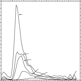
Figure 16.7 Wave spectra of a fully developed sea for di erent wind speeds according to Moskowitz (1964).

Pierson-Moskowitz Spectrum Various idealized spectra are used to answer the question in oceanography and ocean engineering. Perhaps the simplest is that proposed by Pierson and Moskowitz (1964). They assumed that if the wind blew steadily for a long time over a large area, the waves would come into equilibrium with the wind. This is the concept of a fully developed sea. Here, a “long time” is roughly ten-thousand wave periods, and a “large area” is roughly five-thousand wave lengths on a side.

To obtain a spectrum of a fully developed sea, they used measurements of waves made by accelerometers on British weather ships in the north Atlantic. First, they selected wave data for times when the wind had blown steadily for long times over large areas of the north Atlantic. Then they calculated the wave spectra for various wind speeds (figure 16.7), and they found that the function

was a good fit to the observed spectra, where ω = 2πf , f is the wave frequency

in Hertz, α = 8.1 × 10−3, β = 0.74 , ω0 = g/U19.5 and U19.5 is the wind speed at a height of 19.5 m above the sea surface, the height of the anemometers on

the weather ships used by Pierson and Moskowitz (1964).

For most airflow over the sea the atmospheric boundary layer has nearly