- •Preface
- •1 A Voyage of Discovery
- •1.2 Goals
- •1.3 Organization
- •1.4 The Big Picture
- •1.5 Further Reading
- •2 The Historical Setting
- •2.2 Eras of Oceanographic Exploration
- •2.3 Milestones in the Understanding of the Ocean
- •2.4 Evolution of some Theoretical Ideas
- •2.5 The Role of Observations in Oceanography
- •2.6 Important Concepts
- •3 The Physical Setting
- •3.1 Ocean and Seas
- •3.2 Dimensions of the ocean
- •3.3 Sea-Floor Features
- •3.4 Measuring the Depth of the Ocean
- •3.5 Sea Floor Charts and Data Sets
- •3.6 Sound in the Ocean
- •3.7 Important Concepts
- •4.1 The Earth in Space
- •4.2 Atmospheric Wind Systems
- •4.3 The Planetary Boundary Layer
- •4.4 Measurement of Wind
- •4.5 Calculations of Wind
- •4.6 Wind Stress
- •4.7 Important Concepts
- •5 The Oceanic Heat Budget
- •5.1 The Oceanic Heat Budget
- •5.2 Heat-Budget Terms
- •5.3 Direct Calculation of Fluxes
- •5.4 Indirect Calculation of Fluxes: Bulk Formulas
- •5.5 Global Data Sets for Fluxes
- •5.6 Geographic Distribution of Terms
- •5.7 Meridional Heat Transport
- •5.8 Variations in Solar Constant
- •5.9 Important Concepts
- •6.2 Definition of Temperature
- •6.4 The Oceanic Mixed Layer and Thermocline
- •6.5 Density
- •6.6 Measurement of Temperature
- •6.7 Measurement of Conductivity or Salinity
- •6.8 Measurement of Pressure
- •6.10 Light in the Ocean and Absorption of Light
- •6.11 Important Concepts
- •7.1 Dominant Forces for Ocean Dynamics
- •7.2 Coordinate System
- •7.3 Types of Flow in the ocean
- •7.4 Conservation of Mass and Salt
- •7.5 The Total Derivative (D/Dt)
- •7.6 Momentum Equation
- •7.7 Conservation of Mass: The Continuity Equation
- •7.8 Solutions to the Equations of Motion
- •7.9 Important Concepts
- •8.2 Turbulence
- •8.3 Calculation of Reynolds Stress:
- •8.4 Mixing in the Ocean
- •8.5 Stability
- •8.6 Important Concepts
- •9 Response of the Upper Ocean to Winds
- •9.1 Inertial Motion
- •9.2 Ekman Layer at the Sea Surface
- •9.3 Ekman Mass Transport
- •9.4 Application of Ekman Theory
- •9.5 Langmuir Circulation
- •9.6 Important Concepts
- •10 Geostrophic Currents
- •10.1 Hydrostatic Equilibrium
- •10.2 Geostrophic Equations
- •10.3 Surface Geostrophic Currents From Altimetry
- •10.4 Geostrophic Currents From Hydrography
- •10.5 An Example Using Hydrographic Data
- •10.6 Comments on Geostrophic Currents
- •10.7 Currents From Hydrographic Sections
- •10.8 Lagrangian Measurements of Currents
- •10.9 Eulerian Measurements
- •10.10 Important Concepts
- •11.2 Western Boundary Currents
- •11.4 Observed Surface Circulation in the Atlantic
- •11.5 Important Concepts
- •12 Vorticity in the Ocean
- •12.2 Conservation of Vorticity
- •12.4 Vorticity and Ekman Pumping
- •12.5 Important Concepts
- •13.2 Importance of the Deep Circulation
- •13.3 Theory for the Deep Circulation
- •13.4 Observations of the Deep Circulation
- •13.5 Antarctic Circumpolar Current
- •13.6 Important Concepts
- •14 Equatorial Processes
- •14.1 Equatorial Processes
- •14.6 Important Concepts
- •15 Numerical Models
- •15.2 Numerical Models in Oceanography
- •15.3 Global Ocean Models
- •15.4 Coastal Models
- •15.5 Assimilation Models
- •15.6 Coupled Ocean and Atmosphere Models
- •15.7 Important Concepts
- •16 Ocean Waves
- •16.1 Linear Theory of Ocean Surface Waves
- •16.2 Nonlinear waves
- •16.3 Waves and the Concept of a Wave Spectrum
- •16.5 Wave Forecasting
- •16.6 Measurement of Waves
- •16.7 Important Concepts
- •17 Coastal Processes and Tides
- •17.1 Shoaling Waves and Coastal Processes
- •17.2 Tsunamis
- •17.3 Storm Surges
- •17.4 Theory of Ocean Tides
- •17.5 Tidal Prediction
- •17.6 Important Concepts
- •References
12.4. VORTICITY AND EKMAN PUMPING |
205 |
|
Westerlies |
|
ζ |
ζ |
τ |
|
τ |
|
|
+ |
|
|
ζ |
|
ζ |
Trades |
|
|
|
+
Westerlies
ζ b
ζ
Trades
+
ζ τ
ζ
Figure 12.5 The balance of potential vorticity can clarify why western boundary currents are necessary. Left: Vorticity input by the wind ζτ balances the change in relative vorticity ζ in the east as the flow moves southward and f decreases. The two do not balance in the west where ζ must decrease as the flow moves northward and f increases. Right: Vorticity in the west is balanced by relative vorticity ζb generated by shear in the western boundary current.
12.4Vorticity and Ekman Pumping
Rotation places another very interesting constraint on the geostrophic flow field. To help understand the constraints, let’s first consider flow in a fluid with constant rotation. Then we will look into how vorticity constrains the flow of a fluid with rotation that varies with latitude. An understanding of the constraints leads to a deeper understanding of Sverdrup’s and Stommel’s results discussed in the last chapter.
Fluid dynamics on the f Plane: the Taylor-Proudman Theorem The influence of vorticity due to earth’s rotation is most striking for geostrophic flow of a fluid with constant density ρ0 on a plane with constant rotation f = f0. From Chapter 10, the three components of the geostrophic equations (10.4) are:
f v =
1 ∂p
ρ0 ∂x
f u = − 1 ∂p ρ0 ∂y
g = − 1 ∂p ρ0 ∂z
and the continuity equations (7.19) is:
0 = ∂u∂x + ∂v∂y + ∂w∂z
Taking the z derivative of (12.13a) and using (12.13c) gives:
(12.13a)
(12.13b)
(12.13c)
(12.13d)
−f0 ∂z |
= −ρ0 |
|
∂z |
∂x |
= |
∂x |
−ρ0 |
|
∂z |
= |
∂x = 0 |
|||
|
∂v |
1 |
|
∂ |
|
∂p |
|
∂ |
1 |
|
∂p |
|
∂g |
|
f0 |
∂v |
= 0 |
|
|
|
|
|
|
|
|
|
|
|
|
|
|
|
|
|
|
|
|
|
|
|
|
|
||
∂z |
|
|
|
|
|
|
|
|
|
|
|
|
||
|
∂v |
= 0 |
|
|
|
|
|
|
|
|
|
|
|
|
|
|
|
|
|
|
|
|
|
|
|
|
|
||
∂z |
|
|
|
|
|
|
|
|
|
|
|
|
206 |
CHAPTER 12. VORTICITY IN THE OCEAN |
Similarly, for the u-component of velocity (12.13b). Thus, the vertical derivative of the horizontal velocity field must be zero.
|
∂u |
= |
∂v |
= 0 |
(12.14) |
|
∂z |
∂z |
|||
|
|
|
|
This is the Taylor-Proudman Theorem, which applies to slowly varying flows in a homogeneous, rotating, inviscid fluid. The theorem places strong constraints on the flow:
If therefore any small motion be communicated to a rotating fluid the resulting motion of the fluid must be one in which any two particles originally in a line parallel to the axis of rotation must remain so, except for possible small oscillations about that position—Taylor (1921).
Hence, rotation greatly sti ens the flow! Geostrophic flow cannot go over a seamount, it must go around it. Taylor (1921) explicitly derived (12.14) and (12.16) below. Proudman (1916) independently derived the same theorem but not as explicitly.
Further consequences of the theorem can be obtained by eliminating the pressure terms from (12.13a & 12.13b) to obtain:
∂u |
|
∂v |
|
|
∂ |
|
|
1 |
|
∂p |
|
|
|
∂ |
1 |
|
∂p |
|
|
|||||
|
+ |
|
= − |
|
|
|
|
|
|
|
|
|
+ |
|
|
|
|
|
|
(12.15a) |
||||
∂x |
∂y |
∂x |
f0 ρ0 |
|
∂y |
∂y |
f0 ρ0 |
|
∂x |
|||||||||||||||
∂u |
+ |
∂v |
= |
|
1 |
|
− |
|
∂2p |
|
+ |
|
∂2p |
|
|
|
|
|
(12.15b) |
|||||
∂x |
∂y |
f0 ρ0 |
|
∂x ∂y |
|
∂x ∂y |
|
|
|
|||||||||||||||
∂u |
+ |
∂v |
= 0 |
|
|
|
|
|
|
|
|
|
|
|
|
|
|
|
|
|
|
|
(12.15c) |
|
∂x |
∂y |
|
|
|
|
|
|
|
|
|
|
|
|
|
|
|
|
|
|
|
||||
|
|
|
|
|
|
|
|
|
|
|
|
|
|
|
|
|
|
|
|
|
|
|
Because the fluid is incompressible, the continuity equation (12.13d) requires
∂w |
= 0 |
(12.16) |
|
∂z |
|||
|
|
Furthermore, because w = 0 at the sea surface and at the sea floor, if the bottom is level, there can be no vertical velocity on an f –plane. Note that the derivation of (12.16) did not require that density be constant. It requires only slow motion in a frictionless, rotating fluid.
Fluid Dynamics on the Beta Plane: Ekman Pumping If (12.16) is true, the flow cannot expand or contract in the vertical direction, and it is indeed as rigid as a steel bar. There can be no gradient of vertical velocity in an ocean with constant planetary vorticity. How then can the divergence of the Ekman transport at the sea surface lead to vertical velocities at the surface or at the base of the Ekman layer? The answer can only be that one of the constraints used in deriving (12.16) must be violated. One constraint that can be relaxed is the requirement that f = f0.
12.4. VORTICITY AND EKMAN PUMPING |
207 |
Consider then flow on a beta plane. If f = f0 + β y, then (12.15a) becomes:
|
|
∂u |
|
|
∂v |
1 |
|
∂2p |
|
1 ∂2p |
|
β 1 ∂p |
|
|||||||||
|
|
|
|
+ |
|
|
= − |
|
|
|
+ |
|
|
|
− |
|
|
|
|
|
(12.17) |
|
f |
|
∂x |
∂y |
f ρ0 |
|
∂x ∂y |
f ρ0 |
∂x ∂y |
f |
f ρ0 |
∂x |
|||||||||||
∂u |
|
∂v |
|
|
|
|
|
|
|
|
|
|
|
|
|
|
|
|||||
|
+ |
|
= −β v |
|
|
|
|
|
|
|
|
|
|
|
|
(12.18) |
||||||
∂x |
∂y |
|
|
|
|
|
|
|
|
|
|
|
|
where we have used (12.13a) to obtain v in the right-hand side of (12.18). Using the continuity equation, and recalling that β y f0
f0 |
∂wG |
= β v |
(12.19) |
|
∂z |
||||
|
|
|
where we have used the subscript G to emphasize that (12.19) applies to the ocean’s interior, geostrophic flow. Thus the variation of Coriolis force with latitude allows vertical velocity gradients in the geostrophic interior of the ocean, and the vertical velocity leads to north-south currents. This explains why Sverdrup and Stommel both needed to do their calculations on a β-plane.
Ekman Pumping in the Ocean In Chapter 9, we saw that the curl of the wind stress T produced a divergence of the Ekman transports leading to a vertical velocity wE (0) at the top of the Ekman layer. In Chapter 9 we derived
T
wE (0) = −curl (12.20)
ρf
which is (9.30b) where ρ is density and f is the Coriolis parameter. Because the vertical velocity at the sea surface must be zero, the Ekman vertical velocity must be balanced by a vertical geostrophic velocity wG(0).
wE (0) = −wG(0) = −curl |
T |
|
(12.21) |
|
|||
ρf |
Ekman pumping (wE (0)) drives a vertical geostrophic current (−wG(0)) in the ocean’s interior. But why does this produce the northward current calculated by Sverdrup (11.6)? Peter Niiler (1987: 16) gives an explanation.
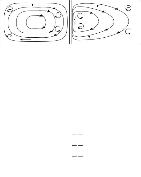
Let us postulate there exists a deep level where horizontal and vertical motion of the water is much reduced from what it is just below the mixed layer [figure 12.6]. . . Also let us assume that vorticity is conserved there (or mixing is small) and the flow is so slow that accelerations over the earth’s surface are much smaller than Coriolis accelerations. In such a situation a column of water of depth H will conserve its spin per unit volume, f /H (relative to the sun, parallel to the earth’s axis of rotation). A vortex column which is compressed from the top by wind-forced sinking (H decreases) and whose bottom is in relatively quiescent water would tend to shorten and slow its spin. Thus because of the curved ocean surface it has to move southward (or extend its column) to regain its spin. Therefore, there should be a massive flow of water at some depth
208
|
|
|
|
|
i n |
d |
s |
|
|
|
|
|
W |
|
|
||
|
|
|
|
|
|
|
||
|
a |
d |
e |
|
|
|
|
|
|
|
|
|
|
|
|||
|
|
|
|
|
|
|
||
|
|
|
|
|
|
|
|
|
r |
|
|
|
|
|
|
|
|
T |
|
|
|
|
|
|
|
|
CHAPTER 12. VORTICITY IN THE OCEAN
North Pole
|
|
|
|
|
s |
|
|
|
|
ie |
|
|
|
|
rl |
|
|
|
|
te |
|
|
|
|
s |
|
|
|
|
e |
|
|
|
|
|
W |
|
|
|
|
|
|
|
|
|
|
|
|
|
ic |
|
|
|
|
|
|
|
|
|
|
|
|
|
|
|
|
ph |
|
|
|
|
|
|
|
o |
|
|
|
|
|
|
|
tr |
|
|
|
|
|
|
|
s |
|
|
|
|
|
|
|
o |
|
|
|
|
|
|
|
e |
|
|
|
or |
|
|
|
|
G |
|
|
|
|
|
|
|
|
|
|
|
ri |
|
||
|
|
|
|
|
te |
|
|
|
|
|
|
In |
|
|
|
||
|
|
|
|
|
|
|
|
|
|
|
|
|
|
|
|
|
|
Figure 12.6 Ekman pumping that produces a downward velocity at the base of the Ekman layer forces the fluid in the interior of the ocean to move southward. See text for why this happens. After Niiler (1987).
below the surface to the south in areas where the surface layers produce a sinking motion and to the north where rising motion is produced. This phenomenon was first modeled correctly by Sverdrup (1947) (after he wrote “ocean”) and gives a dynamically plausible explanation of how wind produces deeper circulation in the ocean.
Peter Rhines (1984) points out that the rigid column of water trying to escape the squeezing imposed by the atmosphere escapes by moving southward. The southward velocity is about 5,000 times greater than the vertical Ekman velocity.
Ekman Pumping: An Example Now let’s see how Ekman pumping drives geostrophic flow in say the central north Pacific (figure 12.7) where the curl of the wind stress is negative. Westerlies in the north drive a southward transport, the trades in the south drive a northward transport. The converging Ekman transports must be balanced by downward geostrophic velocity (12.21).
Because the water near the surface is warmer than the deeper water, the vertical velocity produces a pool of warm water. Much deeper in the ocean, the wind-driven geostrophic current must go to zero (Sverdrup’s hypothesis) and the deep pressure gradients must be zero. As a result, the surface must dome upward because a column of warm water is longer than a column of cold water having the same weight (they must have the same weight, otherwise, the deep pressure would not be constant, and there would be a deep horizontal pressure gradient). Such a density distribution produces north-south pressure gradients at mid depths that must be balanced by east-west geostrophic currents. In short, the divergence of the Ekman transports redistributes mass within the frictionless interior of the ocean leading to the wind-driven geostrophic currents.
Now let’s continue the idea to include the entire north Pacific to see how
12.4. VORTICITY AND EKMAN PUMPING |
209 |
an m k E
|
r |
e |
|
y |
|
a |
|
L |
|
|
e |
d |
|
ra |
|
T |
|
|
s |
d |
|
in |
|
W |
|
|
|
s |
|
|
ie |
|
|
l |
|
r |
|
|
te |
|
|
s |
|
e |
|
|
W |
|
|
ρ1 ρ2
ρ3
ρ4
ρ5 |
North |
|
ρ6 East
Figure 12.7 Winds at the sea surface drive Ekman transports to the right of the wind in this northern hemisphere example (bold arrows in shaded Ekman layer). The converging Ekman transports driven by the trades and westerlies drives a downward geostrophic flow just below the Ekman layer (bold vertical arrows), leading to downward bowing constant density surfaces ρi . Geostrophic currents associated with the warm water are shown by bold arrows. After Tolmazin (1985: 64).
|
|
|
|
|
|
|
Ekman Transports |
Sea Surface Height and |
||||||||||||||
|
|
80º |
|
|
|
|
|
|
|
|
Geostrophic Currents |
|||||||||||
|
|
|
|
|
|
|
|
|
||||||||||||||
|
|
|
|
|
|
|
|
|
|
|
Convergence |
|
|
|
H |
|||||||
|
|
|
Easterlies |
|
|
|
|
|
curlτ < 0 |
|
|
|
|
|
|
|
|
|
|
AK |
||
|
|
|
|
|
|
|
|
|
|
|
|
|
|
|
|
|
|
|||||
|
|
|
|
|
|
|
|
|
|
|
|
|
|
|
|
|
|
|||||
|
|
|
|
|
|
|
|
|
|
|
|
|
|
|
|
|
|
|
||||
|
|
60º |
|
|
|
|
|
|
|
|
|
|
|
|
|
|
|
|
|
|
||
|
|
|
|
|
|
|
|
Divergence |
|
|
|
|
L |
|||||||||
|
|
|
|
|
|
|
|
|
|
|
||||||||||||
|
|
|
|
|
|
|
|
|
|
|
|
|
|
|
||||||||
|
|
|
|
|
|
|
|
|
|
|
|
|
|
|
||||||||
|
|
|
|
|
|
|
|
|
|
|
curlτ > 0 |
|
|
|
|
|
|
|
|
|
|
|
|
|
Westerlies |
|
|
|
|
|
|
|
|
|
|
|
|
|
|
|
|
|
|||
|
|
|
|
|
|
|
|
|
|
|
|
|
|
|
|
|
|
|
||||
|
|
40º |
|
|
|
|
|
|
|
|
|
|
|
|
|
|
|
|
|
|
||
|
|
|
|
|
|
|
|
|
|
|
|
|
|
|
|
|
|
|
|
|||
|
|
|
|
|
|
|
|
|
|
|
Convergence |
|
|
|
H |
|||||||
|
|
|
|
|
|
|
|
|
|
|
|
|
|
|||||||||
|
|
|
|
|
|
|
|
|
|
|
curlτ < 0 |
|
|
|
|
|
|
|
|
|
|
|
|
|
|
|
|
|
|
|
|
|
|
|
|
|
|
|
|
|
|
|
|
|
|
|
|
20º |
|
|
|
|
|
|
|
|
|
|
|
|
|
|
|
|
|
NEC |
||
|
|
|
|
|
|
|
|
|
|
|
|
|
|
|
|
|
|
|
||||
|
|
|
|
|
|
|
|
|
|
|
|
|
|
|
|
|
|
|
||||
|
|
|
|
|
|
|
|
|
|
|
|
|
|
|
|
|
|
|
|
|
|
|
|
|
|
Trades |
|
|
|
|
Divergence |
|
|
|
|
|
|
|
|
||||||
|
|
|
|
|
|
|
|
|
|
|
|
|
|
|
|
|
|
|||||
|
|
|
|
|
|
|
|
|
|
|
|
|
|
|
L |
|||||||
|
|
|
|
|
|
|
|
|
|
|
curlτ > 0 |
|
|
|
|
|
|
|
|
|
|
NECC |
|
|
|
|
|
|
|
|
|
|
|
|
|
|
|
|
|
|
|
|
|
||
|
|
|
|
|
|
|
|
|
|
|
Convergence |
|
|
|
|
|
|
|
|
|
||
|
|
|
|
|
|
|
|
|
|
|
|
|
|
|
|
|
|
|
|
|
||
|
|
|
|
|
|
|
|
|
|
|
|
|
|
H |
||||||||
-4 |
0 |
4 |
|
|
|
|||||||||||||||||
curlτ < 0 |
|
|
|
|
||||||||||||||||||
|
|
|
|
|
|
|
|
|
|
|
|
|
|
|
|
|
|
|
|
|
|
Mean Wind Speed (m/s)
Figure 12.8 An example of how winds produce geostrophic currents running upwind. Ekman transports due to winds in the north Pacific (Left) lead to Ekman pumping (Center), which sets up north-south pressure gradients in the upper ocean. The pressure gradients are balanced by the Coriolis force due to east-west geostrophic currents (Right). Horizontal lines indicate regions where the curl of the zonal wind stress changes sign. AK: Alaskan Current, NEC: North Equatorial Current, NECC: North Equatorial Counter Current.