

10.7. CURRENTS FROM HYDROGRAPHIC SECTIONS |
171 |
|||||||||||
|
|
|
|
|
|
|
|
|
|
p1 |
|
|
|
|
z |
v |
2 |
|
v1 |
|
|
p |
2 |
Northern |
|
|
|
|
|
|
|
|
|
|
|
|
|
Hemisphere |
|
Level |
|
β2 |
|
β |
1 |
|
|
p |
3 |
|
|
|
|
|
|
|
|
|
|
|
|
|
||
Surface |
|
|
|
|
|
|
|
|
|
|
|
|
|
|
|
|
|
|
|
ρ1 |
|
|
|
|
|
|
|
|
|
ρ2 |
|
|
|
|
|
p |
4 |
|
|
|
|
|
|
|
|
|
|
|
|
|
|
|
|
|
|
|
γ |
|
|
|
|
|
|
|
|
|
|
|
|
|
|
|
|
x |
Interface |
||
|
|
|
|
|
|
|
|
|
|
|
|
|
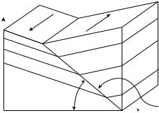
Figure 10.11 Slopes β of the sea surface and the slope γ of the interface between two homogeneous, moving layers, with density ρ1 and ρ2 in the northern hemisphere. After Neumann and Pierson (1966: 166)
10.7Currents From Hydrographic Sections
Lines of hydrographic data along ship tracks are often used to produce contour plots of density in a vertical section along the track. Cross-sections of currents sometimes show sharply dipping density surfaces with a large contrast in density on either side of the current. The baroclinic currents in the section can be estimated using a technique first proposed by Margules (1906) and described by Defant (1961: 453). The technique allows oceanographers to estimate the speed and direction of currents perpendicular to the section by a quick look at the section.
To derive Margules’ equation, consider the slope ∂z/∂x of a stationary interface between two water masses with densities ρ1 and ρ2 (see figure 10.11). To calculate the change in velocity across the interface we assume homogeneous layers of density ρ1 < ρ2 both of which are in geostrophic equilibrium. Although the ocean does not have an idealized interface that we assumed, and the water masses do not have uniform density, and the interface between the water masses is not sharp, the concept is still useful in practice.
The change in pressure on the interface is:
δp = |
∂p |
δx + |
∂p |
δz, |
(10.18) |
||
∂x |
∂z |
|
|||||
|
|
|
|
||||
and the vertical and horizontal pressure gradients are obtained from (10.6):
|
∂p |
|
||
|
|
= −ρ1g + ρ1f v1 |
(10.19) |
|
|
∂z |
|||
Therefore: |
|
|
|
|
δp1 |
= −ρ1f v1 δx + ρ1g δz |
(10.20a) |
||
δp2 |
= −ρ2f v2 δx + ρ2g δz |
(10.20b) |
||
The boundary conditions require δp1 = δp2 on the interface if the interface is not moving. Equating (10.20a) with (10.20b), dividing by δx, and solving for

172 |
|
CHAPTER 10. |
GEOSTROPHIC CURRENTS |
||||||||||
δz/δx gives: |
|
|
|
|
g |
|
|
ρ2 |
− ρ1 |
|
|
||
|
δx ≡ |
|
|
|
|
|
|
||||||
|
δz |
tan γ = |
f |
|
|
ρ2 v2 |
− ρ1 v1 |
|
|
||||
|
|
|
|
|
|
|
|
|
|||||
Because ρ1 ≈ ρ2, and for small β and γ, |
|
|
(v2 − v1) |
|
|||||||||
|
tan γ ≈ g ρ2 |
−1 |
ρ1 |
(10.21a) |
|||||||||
|
|
|
f |
ρ |
|
|
|
|
|
||||
|
tan β1 = − |
f |
|
|
|
|
|
|
|||||
|
|
v1 |
|
|
|
|
|
(10.21b) |
|||||
|
g |
|
|
|
|
|
|||||||
|
|
|
|
f |
|
|
|
|
|
|
|||
|
tan β2 = − |
|
v2 |
|
|
|
|
|
(10.21c) |
||||
|
g |
|
|
|
|
|
|||||||
where β is the slope of the sea surface, and γ is the slope of the interface between the two water masses. Because the internal di erences in density are small, the slope is approximately 1000 times larger than the slope of the constant pressure surfaces.
Consider the application of the technique to the Gulf Stream (figure 10.8). From the figure: ϕ = 36◦, ρ1 = 1026.7 kg/m3, and ρ2 = 1027.5 kg/m3 at a depth of 500 decibars. If we use the σt = 27.1 surface to estimate the slope between the two water masses, we see that the surface changes from a depth of 350 m to a depth of 650 m over a distance of 70 km. Therefore, tan γ = 4300 × 10−6 = 0.0043, and v = v2 − v1 = −0.38 m/s. Assuming v2 = 0, then v1 = 0.38 m/s. This rough estimate of the velocity of the Gulf Stream compares well with velocity at a depth of 500m calculated from hydrographic data (table 10.4) assuming a level of no motion at 2,000 decibars.
The slope of the constant-density surfaces are clearly seen in figure 10.8. And plots of constant-density surfaces can be used to quickly estimate current directions and a rough value for the speed. In contrast, the slope of the sea surface is 8.4 × 10⁻⁶ or 0.84 m in 100 km if we use data from table 10.4.
Note that constant-density surfaces in the Gulf Stream slope downward to the east, and that sea-surface topography slopes upward to the east. Constant pressure and constant density surfaces have opposite slope.
If the sharp interface between two water masses reaches the surface, it is an oceanic front, which has properties that are very similar to atmospheric fronts.
Eddies in the vicinity of the Gulf Stream can have warm or cold cores (figure 10.12). Application of Margules’ method to these mesoscale eddies gives the direction of the flow. Anticyclonic eddies (clockwise rotation in the northern hemisphere) have warm cores (ρ1 is deeper in the center of the eddy than elsewhere) and the constant-pressure surfaces bow upward. In particular, the sea surface is higher at the center of the ring. Cyclonic eddies are the reverse.
10.8Lagrangian Measurements of Currents
Oceanography and fluid mechanics distinguish between two techniques for measuring currents: Lagrangian and Eulerian. Lagrangian techniques follow a water particle. Eulerian techniques measure the velocity of water at a fixed position.
10.8. LAGRANGIAN MEASUREMENTS OF CURRENTS |
173 |
ρ2
|
p |
0 |
|
|
|
ρ1 |
p |
1 |
|
|
p 2
p 3
p 4
p 5
Warm-core ring
p |
0 |
|
|
p |
1 |
|
|
p |
|
2 |
|
p |
|
3 |
|
p |
|
4 |
|
p |
|
5 |
|


 ρ1
ρ1
ρ2
Cold-core ring
Figure 10.12 Shape of constant-pressure surfaces pi and the interface between two water masses of density ρ1, ρ2 if the upper is rotating faster than the lower. Left: Anticyclonic motion, warm-core eddy. Right: Cyclonic, cold-core eddy. Note that the sea surface p0 slopes up toward the center of the warm-core ring, and the constant-density surfaces slope down toward the center. Circle with dot is current toward the reader, circle with cross is current away from the reader. After Defant (1961: 466).
Basic Technique Lagrangian techniques track the position of a drifter designed to follow a water parcel either on the surface or deeper within the water column. The mean velocity over some period is calculated from the distance between positions at the beginning and end of the period divided by the period. Errors are due to:
1.The failure of the drifter to follow a parcel of water. We assume the drifter stays in a parcel of water, but wind blowing on the surface float of a surface drifter can cause the drifter to move relative to the water.
2.Errors in determining the position of the drifter.
3.Sampling errors. Drifters go only where drifters want to go. And drifters want to go to convergent zones. Hence drifters tend to avoid areas of divergent flow.
Satellite Tracked Surface Drifters Surface drifters consist of a drogue plus a float. Its position is determined by the Argos system on meteorological satellites (Swenson and Shaw, 1990) or calculated from gps data recorded continuously by the buoy and relayed to shore.
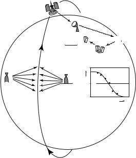
Argos-tracked buoys carry a radio transmitter with a very stable frequency F0. A receiver on the satellite receives the signal and determines the Doppler shift F as a function of time t (figure 10.13). The Doppler frequency is
F = dRdt Fc0 + F0
where R is the distance to the buoy, c is the velocity of light. The closer the buoy to the satellite the more rapidly the frequency changes. When F = F0 the range is a minimum. This is the time of closest approach, and the satellite’s velocity vector is perpendicular to the line from the satellite to the buoy. The time of closest approach and the time rate of change of Doppler frequency at that time gives the buoy’s position relative to the orbit with a 180◦ ambiguity (B and BB in the figure). Because the orbit is accurately known, and because the buoy can be observed many times, its position can be determined without ambiguity.
174 |
CHAPTER 10. GEOSTROPHIC CURRENTS |
E
 K
K
A2
A1
BB |
F F0 |
|
B |
t
Figure 10.13 System Argos uses radio signals transmitted from surface buoys to determine the position of the buoy. A satellite receives the signal from the buoy B. The time rate of change of the signal, the Doppler shift F , is a function of buoy position and distance from the satellite’s track. Note that a buoy at BB would produce the same Doppler shift as the buoy at B. The recorded Doppler signal is transmitted to ground stations E, which relays the information to processing centers A via control stations K. After Dietrich et al. (1980: 149).
The accuracy of the calculated position depends on the stability of the frequency transmitted by the buoy. The Argos system tracks buoys with an accuracy of ±(1–2) km, collecting 1–8 positions per day depending on latitude. Because 1 cm/s ≈ 1 km/day, and because typical values of currents in the ocean range from one to two hundred centimeters per second, this is an very useful accuracy.
Holey-Sock Drifters The most widely used, satellite-tracked drifter is the holey-sock drifter. It consists of a cylindrical drogue of cloth 1 m in diameter by 15 m long with 14 large holes cut in the sides. The weight of the drogue is supported by a float set 3 m below the surface. The submerged float is tethered to a partially submerged surface float carrying the Argos transmitter.
The buoy was designed for the Surface Velocity Program and extensively tested. Niiler et al. (1995) carefully measured the rate at which wind blowing on the surface float pulls the drogue through the water, and they found that the buoy moves 12 ± 9◦ to the right of the wind at a speed
Us = (4.32 ± 0.67×) 10 |
−2 |
U10 |
+ (11.04 ± 1.63) |
D |
(10.22) |
|
DAR |
DAR |
where DAR is the drag area ratio defined as the drogue’s drag area divided by the sum of the tether’s drag area and the surface float’s drag area, and D is the
10.8. LAGRANGIAN MEASUREMENTS OF CURRENTS |
175 |
di erence in velocity of the water between the top of the cylindrical drogue and the bottom. Drifters typically have a DAR of 40, and the drift Us < 1 cm/s for U10 < 10 m/s.
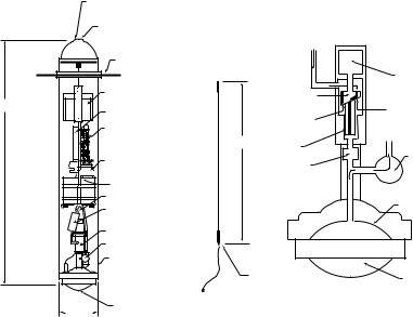
Argo Floats The most widely used subsurface floats are the Argo floats. The floats (figure 10.14) are designed to cycle between the surface and some predetermined depth. Most floats drift for 10 days at a depth of 1 km, sink to 2 km, then rise to the surface. While rising, they profile temperature and salinity as a function of pressure (depth). The floats remains on the surface for a few hours, relays data to shore via the Argos system, then sink again to 1 km. Each float carries enough power to repeat this cycle for several years. The float thus measures currents at 1 km depth and density distribution in the upper ocean. Three thousand Argo floats are being deployed in all parts of the ocean for the Global Ocean Data Assimilation Experiment godae.
|
Argos Antenna Port |
|
Evacuation Port |
|
Camping Disk |
|
Internal Reservoir |
107 cm |
Argos Transmitter |
|
|
|
Controller and |
|
Circuit Boards |
|
Microprocessor |
|
Battery Packs |
|
Pump Battery Packs |
|
Motor |
|
Filter |
|
Hydraulic Pump |
|
Latching Valve |
|
Pressure Case |
|
External Bladder |
|
17cm |
|
From Internal |
|
|
Reservoir |
|
|
|
Motor |
|
Wobble Plate |
|
|
Self-Priming |
Inlet Channel |
|
|
|
|
Channel |
To Internal |
70 cm |
|
Reservoir |
Piston |
|
|
|
|
One-Way |
Latching Valve |
|
|
Check Valve |
|
|
Descending State |
Argos |
Ascending State |
|
Antenna |
||
|
Figure 10.14 The Autonomous Lagrangian Circulation Explorer (ALACE) floats is the prototype for the Argos floats. It measures currents at a depth of 1 km. Left: Schematic of the drifter. To ascend, the hydraulic pump moves oil from an internal reservoir to an external bladder, reducing the drifter’s density. To descend, the latching valve is opened to allow oil to flow back into the internal reservoir. The antenna is mounted to the end cap. Right: Expanded schematic of the hydraulic system. The motor rotates the wobble plate actuating the piston which pumps hydraulic oil. After Davis et al. (1992).
Lagrangian Measurements Using Tracers The most common method for measuring the flow in the deep ocean is to track parcels of water containing molecules not normally found in the ocean. Thanks to atomic bomb tests in the 1950s and the recent exponential increase of chlorofluorocarbons in the atmosphere, such tracers have been introduced into the ocean in large quantities. See §13.4 for a list of tracers used in oceanography. The distribution of trace
176 |
CHAPTER 10. GEOSTROPHIC CURRENTS |
Depth (m)
10 o |
0 o |
10 o |
20 o |
30 o |
40 o |
50 o |
60 o |
70 o |
80 o |
0 |
|
2 |
|
5 |
|
5 6 |
|
H |
3 |
|
|
4 |
|
|
|||||
|
|
|
|
2 |
|||||
|
|
|
|
|
|
4 |
|
|
 1
1
-1000 |
.8 |
|
|
|
8 |
-2000 |
|
|
.8 |
-3000 |
|
|
.8 |
|
1 |
-4000 |
|
Depth (m)
-5000 |
|
|
|
|
|
|
|
|
|
-6000 |
|
|
|
|
|
|
|
|
|
10 o |
0 o |
10 o |
20 o |
30 o |
40 o |
50 o |
60 o |
70 o |
80 o |
0 |
|
|
|
|
|
|
|
|
|
-1000
-2000
-3000
-4000
-5000
-6000 
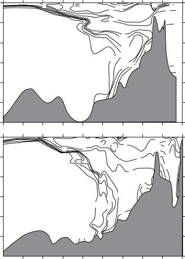
Figure 10.15 Distribution of tritium along a section through the western basins in the north Atlantic, measured in 1972 (Top) and remeasured in 1981 (Bottom). Units are tritium units, where one tritium unit is 1018 (tritium atoms)/(hydrogen atoms) corrected to the activity levels that would have been observed on 1 January 1981. Compare this figure to the density in the ocean shown in figure 13.10. After Toggweiler (1994).
molecules is used to infer the movement of the water. The technique is especially useful for calculating velocity of deep water masses averaged over decades and for measuring turbulent mixing discussed in §8.4.
The distribution of trace molecules is calculated from the concentration of the molecules in water samples collected on hydrographic sections and surveys. Because the collection of data is expensive and slow, there are few repeated sections. Figure 10.15 shows two maps of the distribution of tritium in the north Atlantic collected in 1972–1973 by the Geosecs Program and in 1981, a
10.8. LAGRANGIAN MEASUREMENTS OF CURRENTS |
177 |
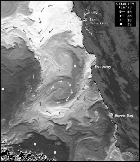
Figure 10.16 Ocean temperature and current patterns are combined in this avhrr analysis. Surface currents were computed by tracking the displacement of small thermal or sediment features between a pair of images. A directional edge-enhancement filter was applied here to define better the di erent water masses. Warm water is shaded darker. From Ocean Imaging, Solana Beach, California, with permission.
decade later. The sections show that tritium, introduced into the atmosphere during the atomic bomb tests in the atmosphere in the 1950s to 1972, penetrated to depths below 4 km only north of 40◦N by 1971 and to 35◦N by 1981. This shows that deep currents are very slow, about 1.6 mm/s in this example.
Because the deep currents are so small, we can question what process are responsible for the observed distribution of tracers. Both turbulent di usion and advection by currents can fit the observations. Hence, does figure 10.15 give mean currents in the deep Atlantic, or the turbulent di usion of tritium?
178 |
CHAPTER 10. GEOSTROPHIC CURRENTS |
Another useful tracer is the temperature and salinity of the water. I will consider these observations in §13.4 where I describe the core method for studying deep circulation. Here, I note that avhrr observations of surface temperature of the ocean are an additional source of information about currents.
Sequential infrared images of surface temperature are used to calculate the displacement of features in the images (figure 10.16). The technique is especially useful for surveying the variability of currents near shore. Land provides reference points from which displacement can be calculated accurately, and large temperature contrasts can be found in many regions in some seasons.
There are two important limitations.
1.Many regions have extensive cloud cover, and the ocean cannot be seen.
2.Flow is primarily parallel to temperature fronts, and strong currents can exist along fronts even though the front may not move. It is therefore essential to track the motion of small eddies embedded in the flow near the front and not the position of the front.
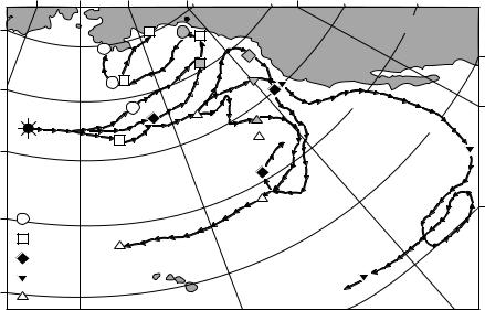
The Rubber Duckie Spill On January 10, 1992 a 12.2-m container with 29,000 bathtub toys, including rubber ducks (called rubber duckies by children) washed overboard from a container ship at 44.7◦N, 178.1◦E (figure 10.17). Ten
|
|
170 o |
-170 o |
-150 o |
-130 o |
-110o |
|
|
|
|
|
Sitka |
North America |
60 o |
|
|
|
|
||
|
|
Bering Sea |
|
|
|
|
50o |
|
|
|
|
|
|
|
|
Origin of |
|
|
|
|
40 |
o |
Toy Spill |
|
|
|
|
|
|
|
|
|
|
|
|
|
|
North Pacific Ocean |
|
|
|
30 o |
1992-94 |
|
|
|
||
|
|
1959-64 |
|
|
|
|
|
|
1984-86 |
|
|
|
|
|
|
1961-63 |
|
Hawaii |
|
|
|
|
|
|
|
||
20 o |
1990-92 |
|
|
10 o |
||
|
|
|
|
|
|
|
Figure 10.17 Trajectories that spilled rubber duckies would have followed had they been spilled on January 10 of di erent years. Five trajectories were selected from a set of 48 simulations of the spill each year between 1946 and 1993. The trajectories begin on January 10 and end two years later (solid symbols). Grey symbols indicate positions on November 16 of the year of the spill. The grey circle gives the location where rubber ducks first came ashore near Sitka in 1992. The code at lower left gives the dates of the trajectories. After Ebbesmeyer and Ingraham (1994).