10.3. SURFACE GEOSTROPHIC CURRENTS FROM ALTIMETRY 155

North Latitude

Figure 10.3 Topex/Poseidon altimeter observations of the Gulf Stream. When the altimeter observations are subtracted from the local geoid, they yield the oceanic topography, which is due primarily to ocean currents in this example. The gravimetric geoid was determined by the Ohio State University from ship and other surveys of gravity in the region. From Center for Space Research, University of Texas.

Typically, sea-surface topography has amplitude of ±1m (figure 10.3). Typical slopes are ∂ζ/∂x ≈ 1–10 microradians for v = 0.1–1.0 m/s at mid latitude.

The height of the geoid, smoothed over horizontal distances greater than roughly 400 km, is known with an accuracy of ±1mm from data collected by the Gravity Recovery and Climate Experiment grace satellite mission.

Satellite Altimetry Very accurate, satellite-altimeter systems are needed for measuring the oceanic topography. The first systems, carried on Seasat, Geosat, ers–1, and ers–2 were designed to measure week-to-week variability of currents. Topex/Poseidon, launched in 1992, was the first satellite designed to make the much more accurate measurements necessary for observing the permanent (timeaveraged) surface circulation of the ocean, tides, and the variability of gyre-scale currents. It was followed in 2001 by Jason and in 2008 by Jason-2.

Because the geoid was not well known locally before about 2004, altimeters were usually flown in orbits that have an exactly repeating ground track. Thus Topex/Poseidon and Jason fly over the same ground track every 9.9156 days. By subtracting sea-surface height from one traverse of the ground track from height measured on a later traverse, changes in topography can be observed without knowing the geoid. The geoid is constant in time, and the subtraction removes the geoid, revealing changes due to changing currents, such as mesoscale eddies, assuming tides have been removed from the data (figure 10.4). Mesoscale variability includes eddies with diameters between roughly 20 and 500 km.

Four-Year Mean Sea-Surface Topography (cm)

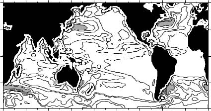
Figure 10.5 Global distribution of time-averaged topography of the ocean from Topex/Poseidon altimeter data from 10/3/92 to 10/6/99 relative to the jgm–3 geoid. Geostrophic currents at the ocean surface are parallel to the contours. Compare with figure 2.8 calculated from hydrographic data. From Center for Space Research, University of Texas.

2.Tracking errors. The satellites carried three tracking systems that enable their position in space, the ephemeris, to be determined with an accuracy of ±(1–3.5) cm.

3.Sampling error. The satellites measure height along a ground track that repeats within ±1 km every 9.9156 days. Each repeat is a cycle. Because currents are measured only along the sub-satellite track, there is a sampling error. The satellite cannot map the topography between ground tracks, nor can they observe changes with periods less than 2 × 9.9156 d (see §16.3).

4.Geoid error. The permanent topography is not well known over distances shorter than a hundred kilometers because geoid errors dominate for short distances. Maps of topography smoothed over greater distances are used to study the dominant features of the permanent geostrophic currents at the sea surface (figure 10.5). New satellite systems grace and champ are measuring earth’s gravity accurately enough that the geoid error is now small enough to ignore over distances greater than 100 km.

Taken together, the measurements of height above the sea and the satellite position give sea-surface height in geocentric coordinates within ±(2–5) cm. Geoid error adds further errors that depend on the size of the area being measured.

10.4Geostrophic Currents From Hydrography

The geostrophic equations are widely used in oceanography to calculate currents at depth. The basic idea is to use hydrographic measurements of temperature, salinity or conductivity, and pressure to calculate the density field of the ocean using the equation of state of sea water. Density is used in (10.7b)

-25 -20 -15 -10 -5 0 5 10 15 20 25 30 cm

Figure 10.6 Time-longitude plot of sea-level anomalies in the Equatorial Pacific observed by Topex/Poseidon during the 1997–1998 El Ni˜no. Warm anomalies are light gray, cold anomalies are dark gray. The anomalies are computed from 10-day deviations from a three-year mean surface from 3 Oct 1992 to 8 Oct 1995. The data are smoothed with a Gaussian weighted filter with a longitudinal span of 5◦and a latitudinal span of 2◦. The annotations on the left are cycles of satellite data. From Center for Space Research, University of Texas.

to calculate the internal pressure field, from which the geostrophic currents are calculated using (10.8a, b). Usually, however, the constant of integration in (10.8) is not known, and only the relative velocity field can be calculated.

At this point, you may ask, why not just measure pressure directly as is done in meteorology, where direct measurements of pressure are used to calculate winds. And, aren’t pressure measurements needed to calculate density from the equation of state? The answer is that very small changes in depth make large changes in pressure because water is so heavy. Errors in pressure caused by errors in determining the depth of a pressure gauge are much larger than the pressure due to currents. For example, using (10.7a), we calculate that the pressure gradient due to a 10 cm/s current at 30◦latitude is 7.5 × 10−3 Pa/m, which is 750 Pa in 100 km. From the hydrostatic equation (10.5), 750 Pa is equivalent to a change of depth of 7.4 cm. Therefore, for this example, we must know the depth of a pressure gauge with an accuracy of much better than 7.4 cm. This is not possible.

Geopotential Surfaces Within the Ocean Calculation of pressure gradients within the ocean must be done along surfaces of constant geopotential just as we calculated surface pressure gradients relative to the geoid when we calculated surface geostrophic currents. As long ago as 1910, Vilhelm Bjerknes (Bjerknes and Sandstrom, 1910) realized that such surfaces are not at fixed heights in the atmosphere because g is not constant, and (10.4) must include the variability of gravity in both the horizontal and vertical directions (Saunders and Fofono , 1976) when calculating pressure in the ocean.

The geopotential Φ is:

Z z

0

Because Φ/9.8 in SI units has almost the same numerical value as height in meters, the meteorological community accepted Bjerknes’ proposal that height be replaced by dynamic meters D = Φ/10 to obtain a natural vertical coordinate. Later, this was replaced by the geopotential meter (gpm) Z = Φ/9.80. The geopotential meter is a measure of the work required to lift a unit mass from sea level to a height z against the force of gravity. Harald Sverdrup, Bjerknes’ student, carried the concept to oceanography, and depths in the ocean are often quoted in geopotential meters. The di erence between depths of constant vertical distance and constant potential can be relatively large. For example, the geometric depth of the 1000 dynamic meter surface is 1017.40 m at the north pole and 1022.78 m at the equator, a di erence of 5.38 m.

Note that depth in geopotential meters, depth in meters, and pressure in decibars are almost the same numerically. At a depth of 1 meter the pressure is approximately 1.007 decibars and the depth is 1.00 geopotential meters.

Equations for Geostrophic Currents Within the Ocean To calculate geostrophic currents, we need to calculate the horizontal pressure gradient within the ocean. This can be done using either of two approaches:

1. Calculate the slope of a constant pressure surface relative to a surface of

constant geopotential. We used this approach when we used sea-surface slope from altimetry to calculate surface geostrophic currents. The sea surface is a constant-pressure surface. The constant geopotential surface was the geoid.

2.Calculate the change in pressure on a surface of constant geopotential. Such a surface is called a geopotential surface.

Figure 10.7. Sketch of geometry used for calculating geostrophic current from hydrography.

Oceanographers usually calculate the slope of constant-pressure surfaces. The important steps are:

1.Calculate di erences in geopotential (ΦA − ΦB ) between two constantpressure surfaces (P1, P2) at hydrographic stations A and B (figure 10.7). This is similar to the calculation of ζ of the surface layer.

2.Calculate the slope of the upper pressure surface relative to the lower.

3.Calculate the geostrophic current at the upper surface relative to the current at the lower. This is the current shear.

4.Integrate the current shear from some depth where currents are known to obtain currents as a function of depth. For example, from the surface downward, using surface geostrophic currents observed by satellite altimetry, or upward from an assumed level of no motion.

To calculate geostrophic currents oceanographers use a modified form of the hydrostatic equation. The vertical pressure gradient (10.6) is written

where α = α(S, t, p) is the specific volume, and (10.12b) follows from (10.11). Di erentiating (10.12b) with respect to horizontal distance x allows the geostrophic balance to be written in terms of the slope of the constant-pressure surface

using (10.6) with f = 2Ω sin φ:

where Φ is the geopotential at the constant-pressure surface.

Now let’s see how hydrographic data are used for evaluating ∂Φ/∂x on a constant-pressure surface. Integrating (10.12b) between two constant-pressure surfaces (P1, P2) in the ocean as shown in figure 10.7 gives the geopotential di erence between two constant-pressure surfaces. At station A the integration

gives:

Z P2A

The specific volume anomaly is written as the sum of two parts:

where α(35, 0, p) is the specific volume of sea water with salinity of 35, temperature of 0◦C, and pressure p. The second term δ is the specific volume anomaly. Using (10.15) in (10.14) gives:

Φ(P1A) − Φ(P2A) = (Φ1 − Φ2)std + ΔΦA

where (Φ1 − Φ2)std is the standard geopotential distance between two constantpressure surfaces P1 and P2, and

Z P2A

is the anomaly of the geopotential distance between the surfaces. It is called the geopotential anomaly. The geometric distance between Φ2 and Φ1 is numerically approximately (Φ2 − Φ1)/g where g = 9.8m/s2 is the approximate value of gravity. The geopotential anomaly is much smaller, being approximately 0.1% of the standard geopotential distance.

Consider now the geopotential anomaly between two pressure surfaces P1 and P2 calculated at two hydrographic stations A and B a distance L meters apart (figure 10.7). For simplicity we assume the lower constant-pressure surface is a level surface. Hence the constant-pressure and geopotential surfaces coincide, and there is no geostrophic velocity at this depth. The slope of the upper surface is

ΔΦB − ΔΦA = slope of constant-pressure surface P2

L

because the standard geopotential distance is the same at stations A and B. The geostrophic velocity at the upper surface calculated from (10.13b) is:

where V is the velocity at the upper geopotential surface. The velocity V is perpendicular to the plane of the two hydrographic stations and directed into the plane of figure 10.7 if the flow is in the northern hemisphere. A useful rule of thumb is that the flow is such that warmer, lighter water is to the right looking downstream in the northern hemisphere.

Note that I could have calculated the slope of the constant-pressure surfaces using density ρ instead of specific volume α. I used α because it is the common practice in oceanography, and tables of specific volume anomalies and computer code to calculate the anomalies are widely available. The common practice follows from numerical methods developed before calculators and computers were available, when all calculations were done by hand or by mechanical calculators with the help of tables and nomograms. Because the computation must be done with an accuracy of a few parts per million, and because all scientific fields tend to be conservative, the common practice has continued to use specific volume anomalies rather than density anomalies.

Barotropic and Baroclinic Flow: If the ocean were homogeneous with constant density, then constant-pressure surfaces would always be parallel to the sea surface, and the geostrophic velocity would be independent of depth. In this case the relative velocity is zero, and hydrographic data cannot be used to measure the geostrophic current. If density varies with depth, but not with horizontal distance, the constant-pressure surfaces are always parallel to the sea surface and the levels of constant density, the isopycnal surfaces. In this case, the relative flow is also zero. Both cases are examples of barotropic flow.

Barotropic flow occurs when levels of constant pressure in the ocean are always parallel to the surfaces of constant density. Note, some authors call the vertically averaged flow the barotropic component of the flow. Wunsch (1996: 74) points out that barotropic is used in so many di erent ways that the term is meaningless and should not be used.

Baroclinic flow occurs when levels of constant pressure are inclined to surfaces of constant density. In this case, density varies with depth and horizontal position. A good example is seen in figure 10.8 which shows levels of constant density changing depth by more than 1 km over horizontal distances of 100 km at the Gulf Stream. Baroclinic flow varies with depth, and the relative current can be calculated from hydrographic data. Note, constant-density surfaces cannot be inclined to constant-pressure surfaces for a fluid at rest.

In general, the variation of flow in the vertical can be decomposed into a barotropic component which is independent of depth, and a baroclinic component which varies with depth.