Cell Terminals

Figure 6.13 A conductivity cell. Current flows through the seawater between platinum electrodes in a cylinder of borosilicate glass 191 mm long with an inside diameter between the electrodes of 4 mm. The electric field lines (solid lines) are confined to the interior of the cell in this design making the measured conductivity (and instrument calibration) independent of objects near the cell. This is the cell used to measure conductivity and salinity shown in figure 6.15. From Sea-Bird Electronics.

surface temperature from the period 1854–1997 using icoads supplemented with satellite data since 1981.

6.7Measurement of Conductivity or Salinity

Conductivity is measured by placing platinum electrodes in seawater and measuring the current that flows when there is a known voltage between the electrodes. The current depends on conductivity, voltage, and volume of sea water in the path between electrodes. If the electrodes are in a tube of nonconducting glass, the volume of water is accurately known, and the current is independent of other objects near the conductivity cell (figure 6.13). The best measurements of salinity from conductivity give salinity with an accuracy of

±0.005.

Before conductivity measurements were widely used, salinity was measured using chemical titration of the water sample with silver salts. The best measurements of salinity from titration give salinity with an accuracy of ±0.02.

Individual salinity measurements are calibrated using standard seawater. Long-term studies of accuracy use data from measurements of deep water masses of known, stable, salinity. For example, Saunders (1986) noted that temperature is very accurately related to salinity for a large volume of water contained in the deep basin of the northwest Atlantic under the Mediterranean outflow. He used the consistency of measurements of temperature and salinity made at many hydrographic stations in the area to estimate the accuracy of temperature, salinity and oxygen measurements. He concluded that the most careful measurements made since 1970 have an accuracy of 0.005 for salinity and 0.005◦C for temperature. The largest source of salinity error was the error in determination of the standard water used for calibrating the salinity measurements.

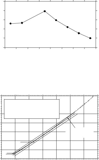
Gouretski and Jancke (1995) estimated accuracyof salinity measurements as a function of time. Using high quality measurements from 16,000 hydrographic stations in the south Atlantic from 1912 to 1991, they estimated accuracy by plotting salinity as a function of temperature using all data collected below 1500 m in twelve regions for each decade from 1920 to 1990. A plot of accuracy as a function of time since 1920 shows consistent improvement in accuracy since 1950 (figure 6.14). Recent measurements of salinity are the most accurate. The

6.8Measurement of Pressure

Pressure is routinely measured by many di erent types of instruments. The SI unit of pressure is the pascal (Pa), but oceanographers normally report pressure in decibars (dbar), where:

because the pressure in decibars is almost exactly equal to the depth in meters. Thus 1000 dbar is the pressure at a depth of about 1000 m.

Strain Gage This is the simplest and cheapest instrument, and it is widely used. Accuracy is about ±1%.

Vibratron Much more accurate measurements of pressure can be made by measuring the natural frequency of a vibrating tungsten wire stretched in a magnetic field between diaphragms closing the ends of a cylinder. Pressure distorts the diaphragm, which changes the tension on the wire and its frequency. The frequency can be measured from the changing voltage induced as the wire vibrates in the magnetic field. Accuracy is about ±0.1%, or better when temperature controlled. Precision is 100–1000 times better than accuracy. The instrument is used to detect small changes in pressure at great depths. Snodgrass (1964) obtained a precision equivalent to a change in depth of ±0.8 mm at a depth of 3 km.

Quartz crystal Very accurate measurements of pressure can also be made by measuring the natural frequency of a quartz crystal cut for minimum temperature dependence. The best accuracy is obtained when the temperature of the crystal is held constant. The accuracy is ±0.015%, and precision is ±0.001% of full-scale values.

Quartz Bourdon Gage has accuracy and stability comparable to quartz crystals. It too is used for long-term measurements of pressure in the deep sea.

6.9 Measurement of Temperature and Salinity with Depth

Temperature, salinity, and pressure are measured as a function of depth using various instruments or techniques, and density is calculated from the measurements.

Bathythermograph (BT) was a mechanical device that measured temperature vs depth on a smoked glass slide. The device was widely used to map the thermal structure of the upper ocean, including the depth of the mixed layer before being replaced by the expendable bathythermograph in the 1970s.

Expendable Bathythermograph (XBT) is an electronic device that measures temperature vs depth using a thermistor on a free-falling streamlined weight. The thermistor is connected to an ohm-meter on the ship by a thin copper wire that is spooled out from the sinking weight and from the moving ship. The xbt is now the most widely used instrument for measuring the thermal structure of the upper ocean. Approximately 65,000 are used each year.

Figure 6.16 Left A CTD ready to be lowered over the side of a ship. From Davis (1987). Right Nansen water bottles before (I), during (II), and after (III) reversing. Both instruments are shown at close to the same scale. After Defant (1961: 33).

The streamlined weight falls through the water at a constant velocity. So depth can be calculated from fall time with an accuracy of ±2%. Temperature accuracy is ±0.1◦C. And, vertical resolution is typically 65 cm. Probes reach to depths of 200 m to 1830 m depending on model.

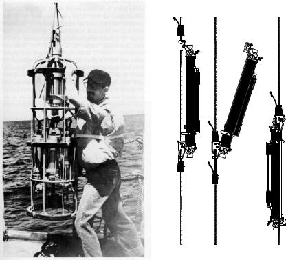
Nansen Bottles (figure 6.16) were deployed from ships stopped at hydrographic stations. Hydrographic stations are places where oceanographers measure water properties from the surface to some depth, or to the bottom, using instruments lowered from a ship. Usually 20 bottles were attached at intervals of a few tens to hundreds of meters to a wire lowered over the side of the ship. The distribution with depth was selected so that most bottles are in the upper layers of the water column where the rate of change of temperature in the vertical is greatest. A protected reversing thermometer for measuring temperature was attached to each bottle along with an unprotected reversing thermometer for measuring depth. The bottle contains a tube with valves on each end to collect sea water at depth. Salinity was determined by laboratory analysis of water sample collected at depth.

After bottles had been attached to the wire and all had been lowered to their selected depths, a lead weight was dropped down the wire. The weight