

- •TABLE OF CONTENTS
- •Chapter 1 INTRODUCTION
- •The es-ice Environment
- •es-ice Meshing Capabilities
- •Tutorial Structure
- •Trimming Tutorial Overview
- •Required Files
- •Trimming Tutorial files
- •Automatic 2D Tutorial files
- •Wall Temperature Tutorial files
- •Mesh Replacement Tutorial files
- •Multiple Cylinder Tutorial files
- •Closed-Cycle Tutorial files
- •Sector Tutorial files
- •Two-Stroke Tutorial files
- •Mapping Tutorial files
- •ELSA Tutorial files
- •Chapter 2 SURFACE PREPARATION IN STAR-CCM+
- •Importing and Scaling the Geometry
- •Creating Features
- •Defining Surfaces
- •Remeshing and Exporting the Geometry
- •Chapter 3 GEOMETRY IMPORT AND VALVE WORK
- •Importing the Surfaces
- •Modelling the Valves
- •Saving the Model
- •Chapter 4 MESHING WITH THE TRIMMING METHOD
- •Modifying Special Cell Sets in the Geometry
- •Defining Flow Boundaries
- •Creating the 2D Base Template
- •Creating the 3D Template
- •Trimming the 3D Template to the Geometry
- •Improving cell connectivity
- •Assembling the Trimmed Template
- •Running Star Setup
- •Saving the Model
- •Chapter 5 CREATING AND CHECKING THE MESH
- •Chapter 6 STAR SET-UP in es-ice
- •Load Model
- •Analysis Set-up
- •Valve Lifts
- •Assembly
- •Combustion
- •Initialization
- •Cylinder
- •Port 1 and Port 2
- •Boundary Conditions
- •Cylinder
- •Port and Valve 1
- •Port and Valve 2
- •Global settings
- •Post Set-up
- •Cylinder
- •Port 1 and Port 2
- •Global settings
- •Time Step Control
- •Write Data
- •Saving the Model
- •Chapter 7 STAR SET-UP in pro-STAR
- •Using the es-ice Panel
- •Setting Solution and Output Controls
- •File Writing
- •Chapter 8 RUNNING THE STAR SOLVER
- •Running in Serial Mode
- •Running in Parallel Mode
- •Running in Parallel on Multiple Nodes
- •Running in Batch
- •Restarting the Analysis
- •Chapter 9 POST-PROCESSING: GENERAL TECHNIQUES
- •Creating Plots with the es-ice Graph Tool
- •Calculating Apparent Heat Release
- •Plotting an Indicator Diagram
- •Calculating Global Engine Quantities
- •Creating a Velocity Vector Display
- •Creating an Animation of Fuel Concentration
- •Creating an Animation of Temperature Isosurfaces
- •Chapter 10 USING THE AUTOMATIC 2D TEMPLATE
- •Importing the Geometry Surface
- •Defining Special Cell Sets in the Geometry
- •Modelling the Valves
- •Creating the Automatic 2D Template
- •Refining the 2D Template Around the Injector
- •Adding Features to the Automatic 2D Template
- •Using Detailed Automatic 2D Template Parameters
- •Saving the es-ice Model File
- •Chapter 11 MULTIPLE-CYCLE ANALYSIS
- •Setting Up Multiple Cycles in es-ice
- •Setting Up Multiple Cycles in pro-STAR
- •Chapter 12 HEAT TRANSFER ANALYSIS
- •Resuming the es-ice Model File
- •Mapping Wall Temperature
- •Exporting Wall Heat Transfer Data
- •Saving the es-ice Model File
- •Cycle-averaging Wall Heat Transfer Data
- •Post-processing Wall Heat Transfer Data in pro-STAR
- •Plotting average wall boundary temperatures
- •Plotting average heat transfer coefficients
- •Plotting average near-wall gas temperature at Y-plus=100
- •Mapping Heat Transfer Data to an Abaqus Model via STAR-CCM+
- •Chapter 13 MESH REPLACEMENT
- •Preparing the File Structure
- •Rebuilding the Dense Mesh
- •Creating Ahead Files for the Dense Mesh
- •Defining Mesh Replacements
- •Setting Up Mesh Replacement in pro-STAR
- •Setting up the coarse model
- •Setting up the dense model
- •Chapter 14 MULTIPLE CYLINDERS
- •Resuming the es-ice Model File
- •Making, Cutting and Assembling the Template
- •Setting Up Multiple Cylinders
- •Checking the Computational Mesh
- •STAR Set-Up in es-ice
- •Analysis set-up
- •Assembly
- •Combustion
- •Initialization
- •Boundary Conditions
- •Post Setup
- •Time Step Control
- •Write Data
- •Saving the es-ice Model File
- •Importing the Geometry
- •Generating the Closed-Cycle Polyhedral Mesh
- •Assigning shells to geometry cell sets
- •Specifying General, Events and Cylinder parameters
- •Creating a spray-optimised mesh zone
- •Importing a user intermediate surface
- •Checking the spray-optimised zone
- •Creating the closed-cycle polyhedral mesh
- •Running Star Setup
- •Creating and checking the computational mesh
- •Saving the Model File
- •Chapter 16 DIESEL ENGINE: SECTOR MODEL
- •Importing the Bowl Geometry
- •Defining the Bowl Shape
- •Defining the Fuel Injector
- •Creating the 2D Template
- •Creating the Sector Mesh
- •Creating and Checking the Mesh
- •Saving the Model
- •Chapter 17 DIESEL ENGINE: STAR SET-UP IN es-ice and pro-STAR
- •STAR Set-up in es-ice
- •Load model
- •Analysis setup
- •Assembly
- •Combustion
- •Initialization
- •Boundary conditions
- •Post setup
- •Time step control
- •Write data
- •Saving the Model File
- •STAR Set-up in pro-STAR
- •Using the es-ice Panel
- •Selecting Lagrangian and Liquid Film Modelling
- •Setting up the Fuel Injection Model
- •Setting up the Liquid Film Model
- •Setting up Analysis Controls
- •Writing the Geometry and Problem Files and Saving the Model
- •Chapter 18 DIESEL ENGINE: POST-PROCESSING
- •Creating a Scatter Plot
- •Creating a Spray Droplet Animation
- •Chapter 19 TWO-STROKE ENGINES
- •Importing the Geometry
- •Meshing with the Trimming Method
- •Assigning shells to geometry cell sets
- •Creating the 2D template
- •Creating the 3D template
- •Trimming the 3D template to the geometry
- •Assembling the trimmed template
- •Running Star Setup
- •Checking the mesh
- •STAR Set-up in es-ice
- •Analysis setup
- •Assembly
- •Combustion
- •Initialization
- •Boundary conditions
- •Post setup
- •Time step control
- •Write data
- •Saving the es-ice Model File
- •Chapter 20 MESHING WITH THE MAPPING METHOD
- •Creating the Stub Surface in the Geometry
- •Creating the 2D Base Template
- •Creating the 3D Template
- •General Notes About Edges and Splines
- •Creating Edges and Splines Near the Valve Seat
- •Creating the Remaining Edges and Splines
- •Creating Patches
- •The Mapping Process
- •Chapter 21 IMPROVING THE MAPPED MESH QUALITY
- •Creating Plastered Cells
- •Chapter 22 PISTON MODELING
- •Meshing the Piston with the Shape Piston Method
- •Chapter 23 ELSA SPRAY MODELLING
- •Importing the Bowl Geometry
- •Defining the Bowl Shape
- •Setting the Events and Cylinder Parameters
- •Creating the Spray Zone
- •Creating the Sector Mesh
- •STAR Set-up in es-ice
- •Load model
- •Analysis setup
- •Assembly
- •Combustion
- •Initialization
- •Boundary Conditions
- •Time step control
- •Write data
- •Saving the Model File
- •STAR Set-up in pro-STAR
- •Using the es-ice panel
- •Activating the Lagrangian model
- •Defining the ELSA scalars
- •Setting up the Lagrangian droplets
- •Defining boundary regions and boundary conditions
- •Setting up analysis controls
- •Adding extended data for the ELSA model
- •Writing the Geometry and Problem Files and Saving the Model
Chapter 23 |
ELSA SPRAY MODELLING |
Chapter 23 ELSA SPRAY MODELLING
The following tutorial data files are used in this chapter:
ELSA/bowl.dbs
ELSA/injector_hole.spl
ELSA/ufile/dropro.f (ufile directory is required)
ELSA/injection.tbl
The model created at the end of this tutorial is saved to file: save_es-ice.ELSA
The ELSA model captures fuel injection to a high degree of detail by utilizing both the Eulerian and Lagrangian simulation approaches in its implementation. The Eulerian part of the model treats the fuel injected from the nozzle as a continuous liquid phase within the solution domain. The Lagrangian part treats the fuel droplets as a set of Lagrangian parcels once they have separated from the liquid fuel stream. This approach allows you to simulate the spray evolution from the injector nozzle without the need for atomization models or droplet size distributions.
The transition from the Eulerian to the Lagrangian treatment occurs when the liquid phase is sufficiently dilute and the droplet size is determined by the liquid/gas interface area density. For more information on the ELSA methodology and implementation, see Chapter 19 in the STAR-CD Supplementary Notes volume.
This tutorial uses a geometry and engine characteristics similar to those for the closed-cycle polyhedral and sector meshing tutorials. However, certain differences have been introduced to make the model suitable for use in an ELSA analysis.
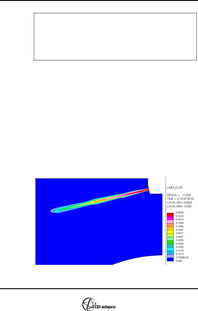
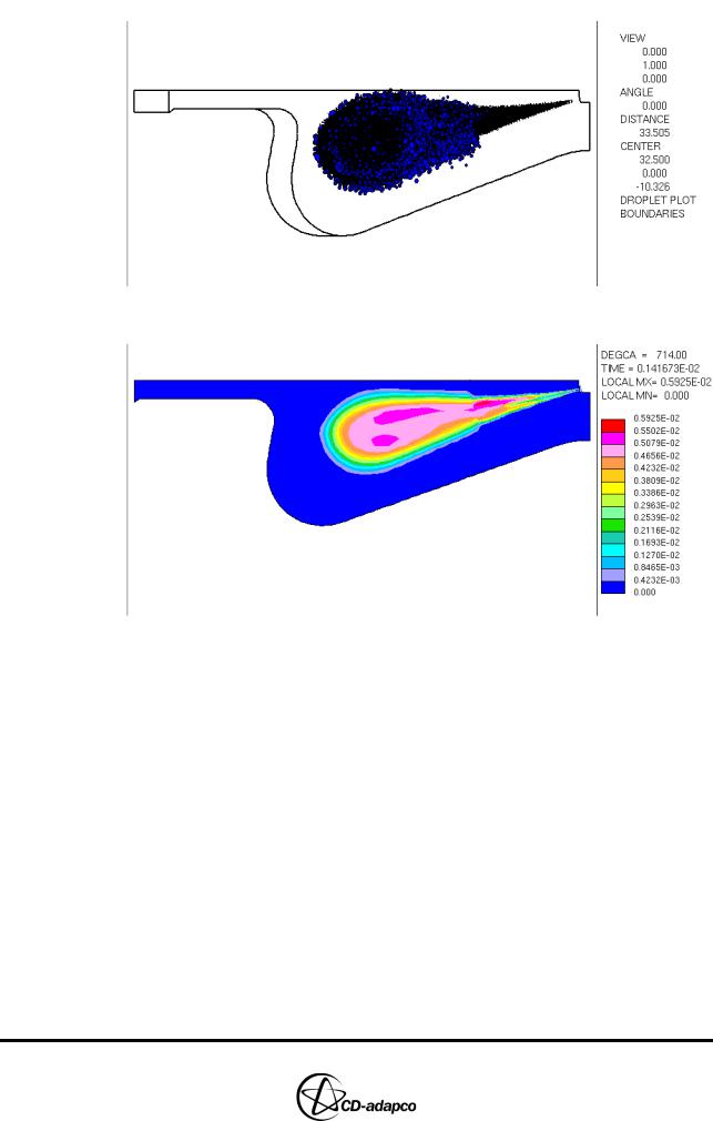
The screen shots below show in some detail the kind of information available with the ELSA model. Figure 23-1 shows the Eulerian liquid fuel being injected from the nozzle into the cylinder. Figure 23-2 shows the Lagrangian droplets generated from the Eulerian phase after break-up. Figure 23-3 shows the fuel vapour generated that participates in the combustion process.
Figure 23-1 ELSA Eulerian liquid fuel stream
Version 4.20 |
23-1 |
ELSA SPRAY MODELLING |
Chapter 23 |
|
|
Figure 23-2 ELSA Lagrangian droplets
Figure 23-3 ELSA fuel vapour distribution
The steps necessary to set up the tutorial are summarised below:
1.Import the piston bowl geometry
2.Create a 2D profile of the piston bowl shape
3.Create the spray zone mesh with a dummy sector mesh
4.Create the cylinder sector mesh and add the spray zone
5.Set-up the Star Controls parameters in es-ice
6.Set up the ELSA model’s analysis control parameters as Extended Data in pro-STAR
23-2 |
Version 4.20 |
Chapter 23 |
ELSA SPRAY MODELLING |
|
Importing the Bowl Geometry |
|
|
Importing the Bowl Geometry
To import the geometry surface mesh:
•Launch es-ice in the usual manner
•In the Select panel, click Read Data
•In the Read Tool, click the ellipsis (...) button next to the DBase box and select bowl.dbs via the file browser
•Click the ellipsis (...) button next to the Get box and select 1 bowl geometry via the database browser
•In the Plot Tool, set the Views option to View 1 -1 1
•Click CPlot to display the imported bowl geometry shown in Figure 23-4
Figure 23-4 Bowl geometry surface
Defining the Bowl Shape
Based on the imported 3D surface mesh, es-ice requires a 2D profile of the bowl shape in order to generate a 2D section of the cylinder. This profile is used at a later stage to trim the 3D template and generate a cylinder volume mesh.
Version 4.20 |
23-3 |
ELSA SPRAY MODELLING |
Chapter 23 |
Setting the Events and Cylinder Parameters |
|
|
|
•Enter the following command to create a spline representing the bowl’s 2D profile:
Spline, 1, RadShell
•In the Plot Tool, set the Views option to View 0 -1 0 to display the spline, as shown in Figure 23-5
Figure 23-5 Displaying the spline representing the bowl
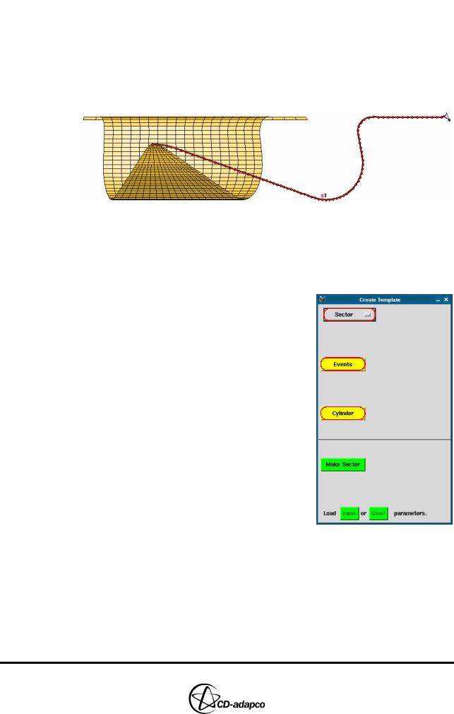
Setting the Events and Cylinder Parameters
The events and cylinder parameters define the engine characteristics and operating conditions. To set these parameters:
•In the Select panel, click Create Template
•In the Create Template panel, select Sector from the drop-down menu
•Click Events
•In the Events parameters panel (see Figure 23-6), set the Crank angle start (deg) to 680
•Set the Crank angle stop (deg) to 800
•Set the Engine RPM to 4000
•Set the Connecting rod length to 270
• Click Ok to accept the settings and close the panel
•In the Create Template panel, click Cylinder
•In the Cylinder parameters panel (see Figure 23-6), set the Piston stroke length to 158.54
•Click Ok to accept the settings and close the panel
23-4 |
Version 4.20 |