Creating the 3D Template

Figure 20-21 General Workspace window: Completed 2D base template

Creating the 3D Template

Now that the 2D template has been created, you can adjust the remaining parameters through the Create Template panel for the third template dimension. Note that, in general, a value of 0 in the parameter boxes denotes a default value calculated by es-ice for the geometry. It is recommended that you initially use as many parameter defaults as possible.

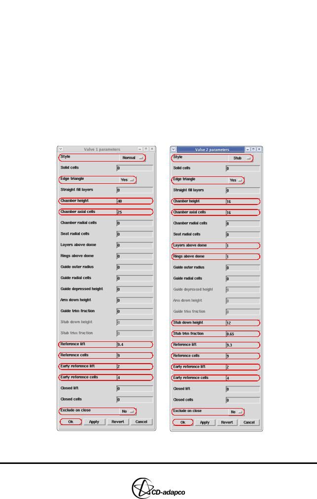
•In the Create Template panel, select Valve 1 from the Valves pull-down menu to bring up the Valve 1 parameters panel. Some key parameters to be specified in this and subsequent panels are indicated in Figure 20-22.

•Since the port associated with this valve will be modelled entirely within es-ice, leave the Style setting to Normal.

•Since Valve 1 has a sizeable chamfer, leave the Edge triangle option to Yes

•The Chamber height, which is the approximate height of the region above the valve (see Figure 20-22), should be specified in model units (millimetres). Enter a value of 40. This value can be obtained using command vdist to pick vertices in a geometry plot of type ‘Hidden’ or using command sxyz in a section plot, as was done earlier for “Creating the Stub Surface in the Geometry”.

•The Chamber axial cells parameter is the number of axial cells throughout that chamber height and should be set to 25 to obtain a reasonable but coarse cell spacing.

•The Chamber radial cells parameter is the number of radial cells in the chamber and this can be left at a value of 0 to accept whatever default value es-ice calculates later to obtain well-proportioned cells in that region.

•By looking at the valve lift files, it can be seen that the maximum valve lift for Valve 1 is close to 9.4 millimetres. Enter a value of 9.4 for Reference lift.

es-ice will try to keep the vertical cell spacing in the valve curtain to a value given by Reference lift divided by Reference cells. For this tutorial example, we will accept a cell spacing of around 1 millimetre:

•Change the Reference cells parameter to 9. Note that an exact value of maximum valve lift is not important. The idea is to assign a value close to the

maximum valve lift and form a ratio with the Reference cells to get the desired cell spacing in the valve curtain at maximum valve lift.

•To improve the mesh density for low valve lifts, enter values of 2 and 4 for the early reference lift and early reference cells, respectively (see Chapter 4, “The Valve parameters panel” in the User Guide for more information).

•At the bottom of the panel, change the Exclude on close parameter to No

•Leave the other parameters at their default values and click Ok

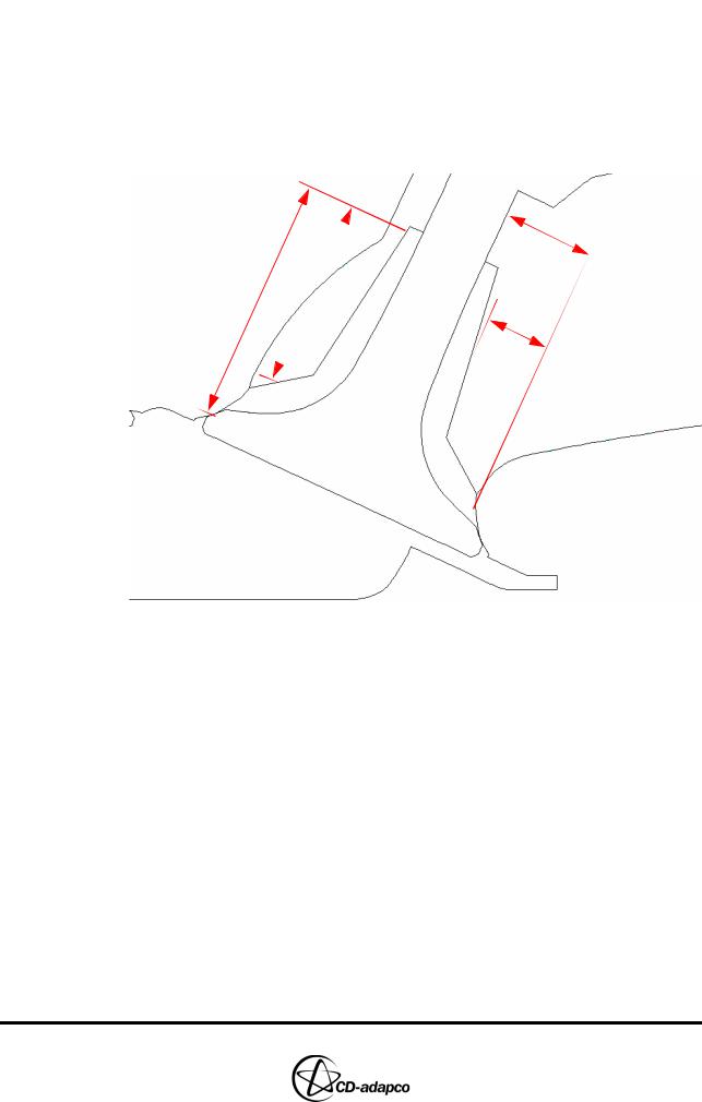
r1

Chamber height

r2/r1 = Stub trim fraction

Figure 20-22 Geometry window: Template parameters for stub

Next, adjust the Valve 2 settings:

•In the Create Template panel, select Valve 2 from the Valves pull-down menu to bring up the Valve 2 parameters panel

•Since the port associated with this valve will be modelled externally by es-ice and a stub surface was created above this valve, change the Style setting to

Stub

•As for Valve 1, leave the Edge triangle option to Yes

•The Chamber height parameter is now the height of the area above the valve, up to the top of the stub. Set this value to 16

•Enter a value of 16 for the Chamber axial cells parameter

•The Chamber radial cells should be specified as 8 to maintain a well-proportioned spacing

•The Stub down height will be the approximate height of the stub step (see Figure 20-22) and a value of 12 can be entered

•The Stub trim fraction will be the ratio of the radial distance of the stub step to the radial distance of the entire stub (see Figure 20-22). Enter a value of 0.65 for this parameter.

Chamber height, Stub down height, Chamber axial cells and Stub trim fraction values should be carefully chosen such that uniform axial and radial cell distribution can be obtained.

Upon closer inspection of the geometry, it will be noticed that Valve 2 is recessed. This appears as a step-like feature around the outside of the valve seat area. To improve the quality of the eventual mapping process, a similar step-like feature can be applied to the template. With a step of this size in the geometry, you can improve the 3D template by adding a single radial cell layer around the valve seat cells. To do this:

•Enter a value of 1 for Layers above dome and Rings above dome. The other values can be left as default.

The panel settings mentioned above are shown in Figure 20-23. When finished entering parameters, click Ok to apply the values and close the panel.

Figure 20-23 Modified 3D parameters for Valve 1 and 2

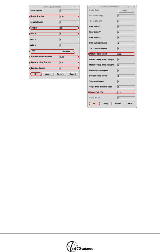
•In the Create Template panel, select Arm 1 from the Arms pull-down menu to bring up the Arm 1 parameters panel (see Figure 4-26 in the User Guide for definitions of the Arm Parameters)

•Enter 0.75 for the Height fraction and 58 for the Length

•The Width layers and Length layers should be left at 0 so that es-ice can calculate default values for these parameters. The default number of Width Layers is generally 1/3 of the number of circumferential layers in the port.

•The intake arm should extend out in the global +x direction from the intake valve, so enter values of 1, 0 and 0 for the Axis X, Axis Y and Axis Z parameters, respectively.

•The intake arm is a siamese-type arm so choose Siamese for the Type parameter. By measurement of the geometry, we can enter values of 0.55, 0.8 and 1 for the Siamese start fraction, Siamese stop fraction and Siamese layers, respectively.

•Click Ok when finished. The completed Arm 1 parameters panel is shown in Figure 20-24.

Since the exhaust arm will not be modelled in es-ice, the parameters for Arm 2 will not be used.

•Next, click the Cylinder button in the Create Template panel to bring up the

Cylinder parameters panel

•Since the stroke in the tutorial example is 68.5 millimetres, enter 68.5 for the

Piston stroke length

The Piston Z at TDC parameter is only used when a flat piston is being modelled. Although this is not the case in this example, it is usually a good idea to check the combustion-dome mapping results before proceeding to model the piston. One method of doing this is to assume a flat piston for the model after the combustion dome mapping is complete:

•Enter a value of -1.5 for Piston Z at TDC to assume a flat piston with a 1.5 millimetre TDC clearance if the real piston geometry is ignored. Note that this parameter will in fact be ignored once the real piston geometry is modelled.

•Leave all other parameters at their default values and then click Ok. The completed Cylinder parameters panel is shown in Figure 20-24.

Figure 20-24 Modified parameters for the Arm 1 and Cylinder parts

•After all parameters have been set, click Make Template in the Create Template panel to make the template and write its information to a file called save_ice by default. This file will be required later, as discussed on page 20-50.

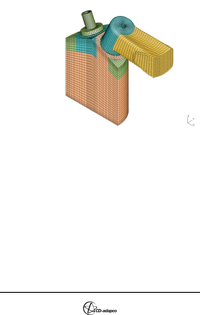
•Click the Read Template button to read the 3D template into the current working session and plot it on the screen, as shown in Figure 20-25.

Note that new local coordinate systems are created (coordinate system ID numbers 13 and 14) which are re-positioned at the bottom of the closed valve and re-oriented so that the x-y rotation is 0. A number of default edges and splines have also been created automatically.

Figure 20-25 Template window: Default 3D template

Next, you need to make a region of the template conform more closely to the spark plug geometry. Because of the relatively coarse template cell size and the relative small size of the spark plug geometry, a few cells from the template in that area will need to be deleted.

After inspecting the spark plug geometry and measuring some vertical distances along the global z-axis, it can be established which cells can be deleted and taken out of the currently active cell set, as shown in Figure 20-26. Because of the simple spark plug geometry, this can be done with cursor picks using the pull-down menus and choosing Sets > Cset > Delete > Cursor.

Figure 20-26 Template window: Template with deleted spark plug cells

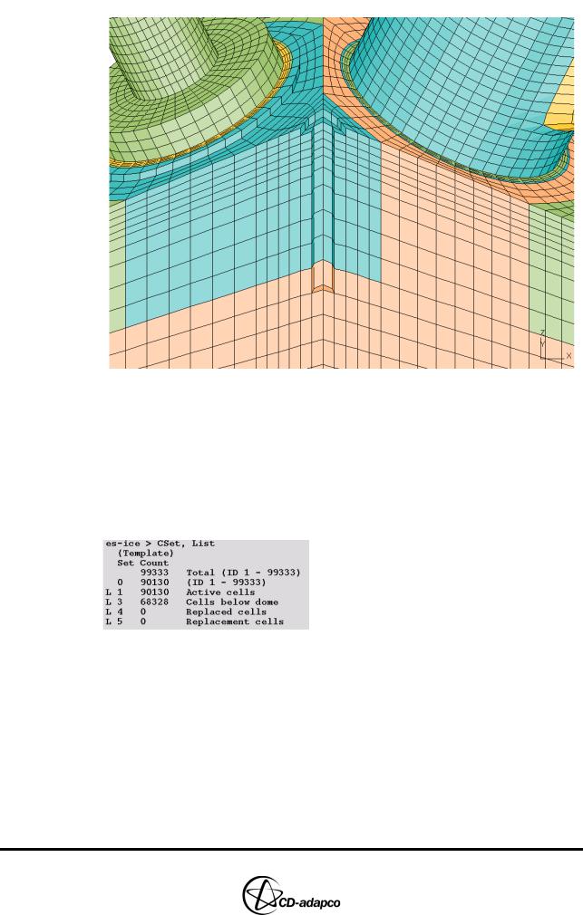
Taking cells out of the currently active cell set is not enough to tell es-ice that you wish to remove these cells from the CFD calculation. Cells in Template Cset 1 are regarded as the cells used in this calculation, so that set must be modified as well.

•Choose Sets > Cset > List from the pull-down menus. A listing of the Template Csets will be displayed (see Figure 20-27), where Cset 0 is the currently active cell set.

After removing spark plug cells

Figure 20-27 A listing of the Template Cset

The “L” on the left-hand side of the above listing indicates a locked cell set and prevents accidental modifications. When the 3D template was first read in and displayed on screen, Template Cset 1 was made the currently active cell set. Now that we have deleted several cells from that set, there are fewer cells in Template Cset 0 then in Template Cset 1. We therefore need to update Template Cset 1 with the cells that we have in the currently active cell set by clicking update cset 1 in the training panel (Note: this button updates Cset 1 of the currently active window so make sure the Template window is active).

es-ice will now exclude the cells in the spark plug cut-out and, after mapping, the mesh will conform to the problem geometry with less distortion than it would have