Chapter 9 POST-PROCESSING: GENERAL TECHNIQUES

The following tutorial data files are used in this chapter:

TRIMMING_TUTORIALS/scalar1.inp

TRIMMING_TUTORIALS/scriptScalar1.sh

TRIMMING_TUTORIALS/isoTemp.inp

TRIMMING_TUTORIALS/scriptIsoTemp.sh

The tutorial in this chapter demonstrates some general post-processing techniques for engine data in both es-ice and pro-STAR.

es-ice can create XY plots from information in either es-ice output data files (es-ice.pos) or external files with data arranged in columns (XYfiles). es-ice can also calculate global engine quantities such as net indicated work, indicated power and indicated mean effective pressure. In addition, it can calculate apparent heat release from pressure data.

pro-STAR can produce two-dimensional and three-dimensional images displaying scalar and vector quantities within the problem geometry. This feature can be used to analyse conditions within the engine cylinder at a given time step. A series of images can also be exported at each time step and then used with third-party software to animate the entire transient analysis results.

The tutorial covers the following topics:

•es-ice:

(a)Creating plots using the es-ice graph tool

(b)Calculating apparent heat release from a pressure plot

(c)Creating a plot displaying pressure against volume (indicator diagram)

(d)Calculating global engine quantities

•pro-STAR:

(a)Creating a two-dimensional display of velocity vectors through the intake valve at maximum valve opening

(b)Creating a three-dimensional animation of fuel distribution within the cylinder over the entire transient solution

(c)Creating a three-dimensional, four-view animation of temperature isosurfaces within the cylinder over the entire transient solution

Examples of post-processing diesel engine models are provided in Chapter 18 of this volume.

Creating Plots with the es-ice Graph Tool

This section details the creation of plots using the es-ice Graph Tool. Two plots are created, one showing temperature against crank angle and the other showing valve curtain flux for both valves. Note that in using an es-ice.pos file, all values are plotted with respect to crank angle.

First, load the output data file (es-ice.pos) into the graph tool, which displays a list of plot data.

•Launch es-ice in the usual manner

•In the Select panel, click Post-process. The Graph Tool is activated by default in the Post-process panel.

•Click the ellipsis (...) button and select es-ice.pos from the file browser

•Click Read

To plot a graph of temperature against crank angle in the es-ice Graph Tool:

•Select item 12 in the list, labelled Temperature: region 1

•Click Plot

Next, modify the data range to suit the expected temperature values, with grid lines and labels added to improve the plot clarity.

•Select the Domain toggle button

•Enter 360 and 1080 in the next two boxes in order to cover an entire engine cycle

•Select Lines, as opposed to Ticks, from the drop-down menu and enter 8 in the adjacent box

•Set Label to Crank Angle

•Select the Range toggle button

•Enter 0 and 2500 in the next two boxes to cover an appropriate data range

•Select Lines (as opposed to Ticks) from the drop-down menu and enter 10 in the adjacent box

•Set Label to Temperature

When complete, the panel will look as shown in Figure 9-1.

Figure 9-1 Temperature against crank angle plot

The Graph Tool can also plot multiple data sets in a single plot. The data set colour can be modified to provide a clear distinction between the sets.

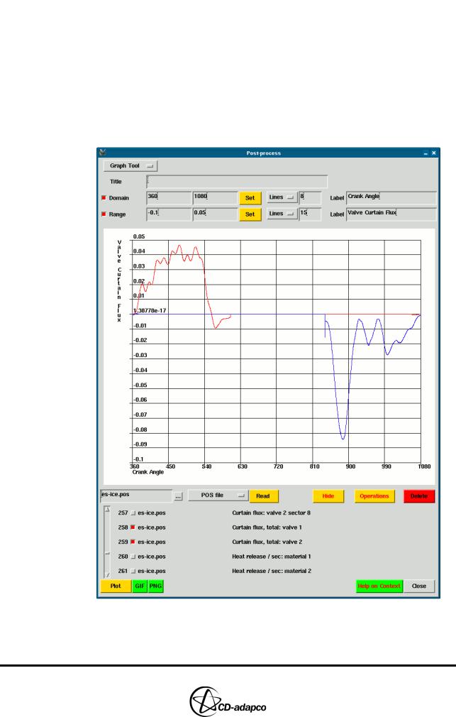
To create a plot of valve curtain flux against crank angle for both valves:

•Deselect the toggle button next to item 12 to clear the temperature data from the graph display

•Select items 258 and 259 in the list, labelled Curtain flux, total: valve 1 and

Curtain flux, total: valve 2, respectively

•Click Plot

•Set the Range to -0.1 and 0.05 to cover a more suitable data range

•Set the number of lines to 15

•Set Label to Valve Curtain Flux

Currently, both data sets are plotted in red. To change the line colour for valve 2:

•Enter the following command in the main es-ice window:

Graph, Format, 259, Color, 4

In this case, 259 defines the data set and 4 changes the colour to blue

•In the Graph Tool, click Plot

When complete, the panel appears as shown in Figure 9-2.

Figure 9-2 Valve curtain flux against crank angle plot for both valves

Plots can also be exported as .gif or .png files by clicking the respective GIF or