General Notes About Edges and Splines

done otherwise.

The user is recommended to save the work up to this point by writing the current working session’s data into a new save_es-ice file using the Write Tool panel. In the tutorial example files, the work up to this point is saved in file

save_es-ice.2-template.

General Notes About Edges and Splines

The template vertices must be moved so that the template acquires the problem geometry’s shape. This movement is accomplished by a sequence of es-ice steps involving feature lines, surfaces and volumes.

The first step involves mapping feature lines in the template called edges to corresponding feature lines in the geometry called splines. Edges are ordered sets of vertices whereas splines are ordered sets of knots that, in general, are smoothly connected. Knots defining a spline may be located on a vertex of the geometry, on a surface shell or on another spline. Thus, splines are more complicated than edges. In the Select panel, an Edge or Spline Tool panel is available to work with these two entity types. Like cells and vertices, splines and edges have ID numbers, can be collected into sets and displayed or hidden with appropriate commands and pull-down menu options.

For every edge in the template, there must be a corresponding spline in the geometry. Edges will be mapped to that spline so that their first and last points coincide and so that the other edge vertices lie on the spline. The vertex spacing can be selected in the Edge or Spline Tool so that the vertices are spaced at equal intervals (linear spacing), proportional to their original spacing in the template (original spacing) or fixed (fixed spacing). Notice that edges and splines can be created in any order but, eventually, corresponding splines and edges must have the same ID number. Exactly how many spline/edge pairs to create and where to create them depends on the complexity of the geometry but also to some extent on the user’s discretion. Note that some splines and edges are generated automatically by es-ice when the 3D template is created.

A number of guidelines concerning splines and edges are listed below:

1.Splines must not intersect. They may be joined end-to-end, but they cannot cross themselves or another spline. Similarly, edges must not intersect.

2.Spline starting and ending points are control points. By breaking one spline into several splines, the user can obtain more control points. The vertices at the ends of the corresponding edges will be mapped to those control points. As indicated previously, intermediate vertices will be spaced either linearly with constant spacing, proportionally to their original template spacing or with fixed spacing, depending on the user’s choice for the edge spacing.

3.Since splines are defined by their knots and knots exist independently of the geometry, there is a variety of pick modes for splines in the Edge or Spline Tool panel. Edges, by contrast, are always placed on vertices of the template and therefore have only one pick mode.

4.To insure that splines connect to each other, the pick mode for the first knot of a new spline should be Knot so that the spline truly begins at the last knot of the previous spline. This will avoid connectivity problems when checks are performed later. Toggling with the right mouse button, the user can change the pick mode for subsequent knots.

Creating Edges and Splines Near the Valve Seat

Let us first focus on the region around the valve seat for Valve 1. It is important that cells in this region are carefully controlled to avoid excessive skew during mesh motion. Typically for each valve, four concentric edges are mapped to four concentric splines in this region.

•In the Geometry window, examine a cross-section of the valve and valve seat region (including a spline plot) by choosing Sets > Sset > All from the pull-down menus. This puts all splines into the current spline set.

•View a section plot through Valve 1 by clicking valve 1 section in the training panel.

•View the section from the direction of the section normal by choosing View Snormal or View 0 1 0 from the Views pull-down menu in the Plot Tool window

•Zoom into the region closer to the other valve

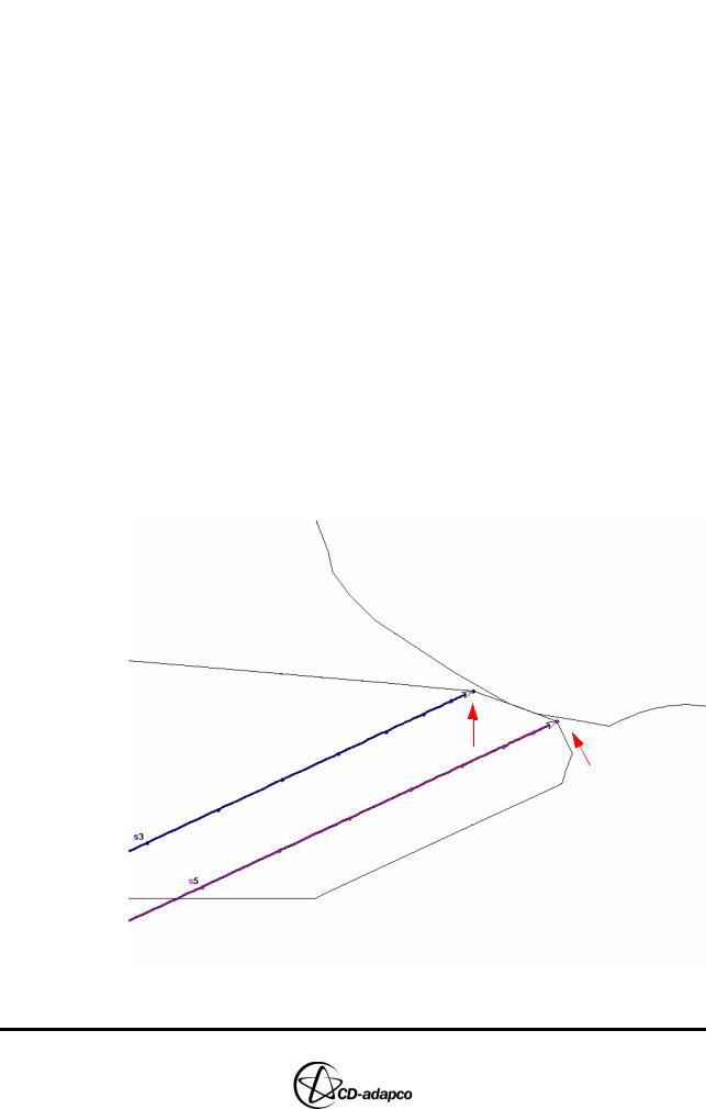
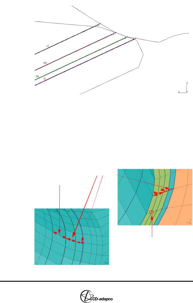
You can see that you need to move two of the automatically-generated splines, spline nos. 3 and 5. This is because these are needed on the outside surface of the problem geometry to control the mesh, not on the valve. Therefore, you need to move the splines to the outside surface. Typically, for steeply angled valves, you can translate the spline at “p4” (spline no. 3) in the global z-direction and the spline at “p3” (spline no. 5) in the local z-direction (see Figure 5-13 on page 5-11 of the User Guide). The easiest way of doing this is to create new splines in the desired locations using the old splines as visual guides.

p4

p5

Figure 20-28 Geometry window: Moving automatically-generated valve splines to the surface

•Click Hidden in the Plot Tool to go back to a ‘hidden’ plot type

We want to create another spline on the surface. This is to be located above the outer, automatically-generated valve spline in the local z-direction, as shown in Figure 20-28.

•View the geometry looking down the +z axis of the local valve coordinate system (ID no. 11) using the following command:

view,0,0,1,11

We will use the Surface option in ‘Pick Knot’ mode. Before doing this, since the valve is very close to the surface in that area, the valve should be deleted from the currently active cell set so that the incorrect surface is not used as a result of tolerance issues.

•Now zoom into the area closer to the other valve

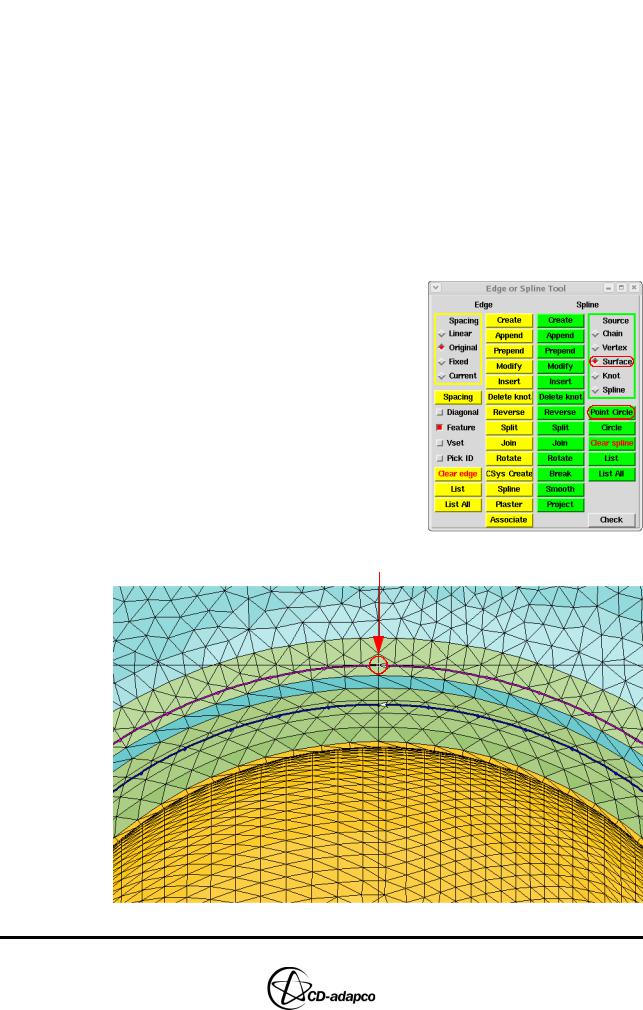
•Starting in ‘Pick Knot’ mode, choose the

Surface option from the Edge or Spline

Tool panel and then click Point Circle.

•Using the existing spline as a visual guide, try to left-click as close to the existing

knot on Spline 5 as possible, as shown in Figure 20-29

•Type q to quit the pick mode and accept the circular spline created

Left-click here

Figure 20-29 Geometry window: Creating a surface spline in the local z-direction

The same thing should be done with the other automatically-generated valve splines:

•View the geometry looking down the +z-axis of the global coordinate system by choosing View 0 0 1 from the Views pull-down menu in the Plot Tool panel

•Zoom into the same area as before, using the Surface option for the ‘Pick Knot’ mode

•Click Point Circle

•Left-click as close as possible to the existing knot of Spline 3

•Type q to quit and accept the newly created circular spline

•Return to the former section view, put all cells into the currently active cell set and plot them, as shown in Figure 20-30. This will enable you to check the new splines visually and decide whether they were created correctly.

Figure 20-30 New splines

Once you verify that everything is correct, the automatically-generated splines are no longer needed. Also, since the edge numbers correspond to these splines on the valve, we would like to renumber the newly created surface splines so that they have the same numbers as their corresponding automatically-generated splines.

•Type the following command: spline,55,renumber,5

The output shown in Figure 20-31 should appear in the es-ice window between the input and output text boxes:

Figure 20-31 Output text in the es-ice window

•Click the Yes option with the mouse or type y

This will not only renumber spline no. 55 as spline no. 5, but also overwrite and destroy the previously-numbered spline no. 5 in the process. The same thing may be done for Spline 56 and 3.

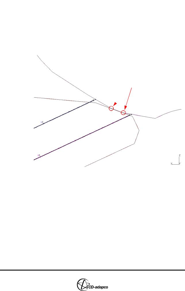
The next step is to add two more concentric splines to indicate the precise location of the valve seat region, as shown in Figure 20-32. These circular splines should be placed at the ends of the shells that define the surface of revolution of the valve seat, in other words the borders of the contact area.

Two additional concentric splines

Figure 20-32 Geometry window: Additional splines needed on each end of the valve seat

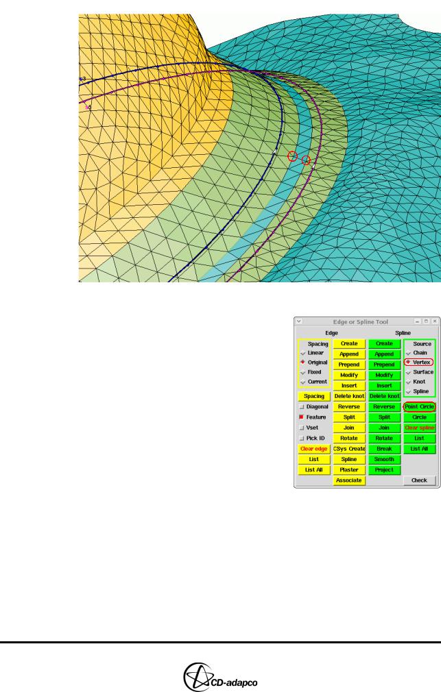
We return to a zoomed hidden view of the previous valve seat area that is closer to the other valve but without the shells for Valve 1. A mesh line that is parallel to the global x-axis is visible in the shells that define the valve curtain region. Note that most of the other circular splines around both valve seat regions have starting/ending knots along this circumferential reference position. When creating new circular splines, it is strongly recommended that you maintain this reference position whenever possible to minimize the possibility of skewing the mesh during the mapping process. Bearing this in mind, note the two vertices shown in Figure 20-33. These lie at the intersection of the reference mesh line parallel to the x-axis and the border of the valve seat shells.

Figure 20-33 Geometry window: Two vertices used to create additional valve splines

•In ‘Pick Knot’ mode, click Vertex in the

Edge or Spline Tool panel

•Click Point Circle to create a circular spline by picking a vertex as the starting/ending knot

•Click one of the two vertices shown in

Figure 20-33 and type q to accept the new spline

•Click Point Circle again, choose the other vertex and then type q to create the other circular spline

A section view through Valve 1, shown in Figure 20-34, will now display the four splines to be used in defining the valve seat region.

Figure 20-34 Geometry window: Four concentric circular splines for valve seat

We will now visualize the four radial cells that will span this region. In the template, there are five edges covering each radial mesh line for those four cells. Since we only need the four splines for this region, one of the edges will need to be cleared. This means that out of the three radial regions defined between the splines, one of them will include two cell layers and the others just one cell layer.

Inspecting the radial distances between the four splines shown on the left-hand side of Figure 20-35, we see that it is best to put two radial cell layers between spline nos. 3 and 55 as these are separated by the largest distance. Then by looking at the five edges that were automatically generated for the valve seat region, we can establish that edge no. 7 (see the right-hand side of Figure 20-35) can be cleared.

One radial cell layer

Two radial cell layers

Edge to clear

Figure 20-35 Geometry (left) and Template (right) windows: Radial cell distribution at the valve seat

To do this:

•Change to the Template panel

•From the menu bar, click Sets > Eset > All

•Click Clear edge and pick a knot on edge no. 7

•Type q to quit the pick mode

Comparison of the corresponding spline and edge numbers in this region will reveal that two of the splines created need to have their ID numbers changed to match their corresponding edges. The spline,#,renum, # command may be used again or, alternatively, the Associate button in the Edge or Spline Tool panel. This is a renumbering function that involves clicking the appropriate splines and edges with the mouse.

•Click Associate. The Template window will become active and the text at the bottom of the window will indicate that we should click on an edge that needs to be associated.

•Left-click on a knot of edge no. 8. es-ice will then make the Geometry window active and the text at the bottom will indicate that we should click on a spline to be associated with the edge we have just picked.

•Left-click on a knot for spline no. 55. This will renumber spline no. 55 to spline no. 8, thus matching the ID number of the edge.

•Similarly, associate Edge 9 with Spline 56

The active window will then be switched to Template and the process repeated until a q is typed to quit. If during the association process the new spline ID is the same as the ID of another spline, the other spline’s ID will be changed to the next available number. Note that the dynamic mode is also available and may be useful in this operation.

The process outlined in this section should be repeated for Valve 2. Note, however, that this valve is recessed and contains a sharp, step-like feature. Therefore, in addition to the actions described so far, two more splines should be created to accommodate it. Since two edges have been generated automatically for that feature, we need to create the two splines corresponding to it, which will be circular and concentric with the other Valve 2 splines. Recall that:

1.The Point Circle option can be used

2.The circumferential reference position of the starting/ending point should be taken into account

3.The ID numbers as well as the directions of corresponding splines and edges should match

The total number of splines created for both valve regions is shown in Figure 20-36.