Exporting Wall Heat Transfer Data

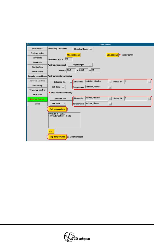
to 1 to select the valve surfaces

•Set Temperature to valves_htx.usr

•Click Get temperature to read the surface mesh and temperature data needed for wall temperature mapping. This step checks the temperature data and boundary surfaces by colouring wall boundaries for which data are available green, and boundaries without data red

•Click Map temperature to map the wall temperature data onto the boundary regions for use as boundary conditions

Figure 12-7 Star controls panel: Boundary conditions view of Global settings

Exporting Wall Heat Transfer Data

To output wall heat transfer data for use in post-processing displays or for a structural analysis:

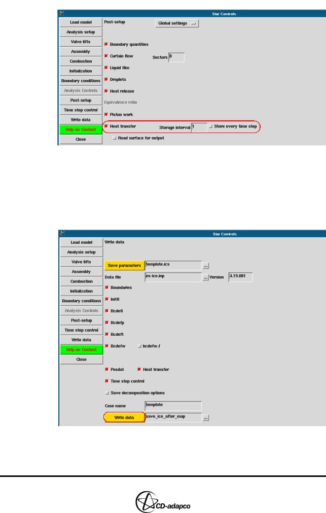
•In the Star Controls panel, open the Post-setup view

•Select Global settings from the drop-down menu

•Select the Heat transfer toggle button, as shown in Figure 12-8

•Ensure that the Storage interval is set to 1 in order to collect data at every crank-angle degree

Figure 12-8 Star controls panel: Post-processing view of Global settings

Finally, use the Write data function to generate the files required for importing the model into pro-STAR.

•In the Star Controls panel, open the Write data view, as shown in Figure 12-9

•Accept the default settings and click Write data to generate the necessary files

Figure 12-9 Star controls panel: Write data view

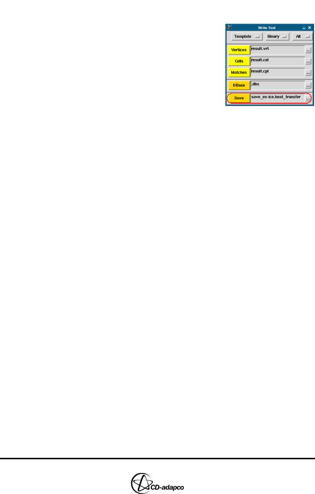
Saving the es-ice Model File

•In the Write Tool, enter save_es-ice.heat_transfer and click

Save

The case set-up can now be finished off in pro-STAR (see Chapter 7) and the analysis run by the STAR solver (see Chapter 8).

Cycle-averaging Wall Heat Transfer Data

When the solver has finished, you can cycle-average the wall heat transfer data by using the Heat Transfer post-processing facilities (see “After completing a simulation, you can use es-ice to generate a presentation that summarises the case features and analysis results. This presentation can be viewed using PowerPoint (Windows) or Open Office (Linux).” on page 12-11 of the User Guide). At this stage, you also need to specify default temperatures and heat transfer coefficients for surfaces that are not permanently exposed to the fluid (and can therefore not be cycle-averaged).

•Load save_es-ice.heat_transfer

•In the Select panel, click Post-process

•Select Heat transfer from the drop-down menu at the top of the Post-process panel, as shown in Figure 12-10

•Click the ellipsis (...) next to the Post data file box and select es-ice_htx.pos from the file browser

•Click Add after selected to add es-ice_htx.pos to the Post data file list

•Click Load post data to load heat transfer data from es-ice_htx.pos. es-ice finds the minimum and maximum crank angles and updates the Crank angle range, in this case 320.1 to 1080 degrees

•Set the Crank angle range minimum to 361 to cover the last engine cycle

•Under Default values for, set the Near wall temperature for each boundary region as follows:

•Liner: 150 C

•Stem 1: 150 C

•Stem 2: 100 C

•Set the Heat transfer coefficient for each boundary region as follows:

•Liner: 1000

•Stem 1: 100

•Stem 2: 100

•Click Cycle average to cycle-average the wall heat transfer data for one cycle

•Set Dbase file to intermediate_bnd.dbs and Dbase ID to 1 to create an