- •TABLE OF CONTENTS
- •Chapter 1 INTRODUCTION
- •The es-ice Environment
- •es-ice Meshing Capabilities
- •Tutorial Structure
- •Trimming Tutorial Overview
- •Required Files
- •Trimming Tutorial files
- •Automatic 2D Tutorial files
- •Wall Temperature Tutorial files
- •Mesh Replacement Tutorial files
- •Multiple Cylinder Tutorial files
- •Closed-Cycle Tutorial files
- •Sector Tutorial files
- •Two-Stroke Tutorial files
- •Mapping Tutorial files
- •ELSA Tutorial files
- •Chapter 2 SURFACE PREPARATION IN STAR-CCM+
- •Importing and Scaling the Geometry
- •Creating Features
- •Defining Surfaces
- •Remeshing and Exporting the Geometry
- •Chapter 3 GEOMETRY IMPORT AND VALVE WORK
- •Importing the Surfaces
- •Modelling the Valves
- •Saving the Model
- •Chapter 4 MESHING WITH THE TRIMMING METHOD
- •Modifying Special Cell Sets in the Geometry
- •Defining Flow Boundaries
- •Creating the 2D Base Template
- •Creating the 3D Template
- •Trimming the 3D Template to the Geometry
- •Improving cell connectivity
- •Assembling the Trimmed Template
- •Running Star Setup
- •Saving the Model
- •Chapter 5 CREATING AND CHECKING THE MESH
- •Chapter 6 STAR SET-UP in es-ice
- •Load Model
- •Analysis Set-up
- •Valve Lifts
- •Assembly
- •Combustion
- •Initialization
- •Cylinder
- •Port 1 and Port 2
- •Boundary Conditions
- •Cylinder
- •Port and Valve 1
- •Port and Valve 2
- •Global settings
- •Post Set-up
- •Cylinder
- •Port 1 and Port 2
- •Global settings
- •Time Step Control
- •Write Data
- •Saving the Model
- •Chapter 7 STAR SET-UP in pro-STAR
- •Using the es-ice Panel
- •Setting Solution and Output Controls
- •File Writing
- •Chapter 8 RUNNING THE STAR SOLVER
- •Running in Serial Mode
- •Running in Parallel Mode
- •Running in Parallel on Multiple Nodes
- •Running in Batch
- •Restarting the Analysis
- •Chapter 9 POST-PROCESSING: GENERAL TECHNIQUES
- •Creating Plots with the es-ice Graph Tool
- •Calculating Apparent Heat Release
- •Plotting an Indicator Diagram
- •Calculating Global Engine Quantities
- •Creating a Velocity Vector Display
- •Creating an Animation of Fuel Concentration
- •Creating an Animation of Temperature Isosurfaces
- •Chapter 10 USING THE AUTOMATIC 2D TEMPLATE
- •Importing the Geometry Surface
- •Defining Special Cell Sets in the Geometry
- •Modelling the Valves
- •Creating the Automatic 2D Template
- •Refining the 2D Template Around the Injector
- •Adding Features to the Automatic 2D Template
- •Using Detailed Automatic 2D Template Parameters
- •Saving the es-ice Model File
- •Chapter 11 MULTIPLE-CYCLE ANALYSIS
- •Setting Up Multiple Cycles in es-ice
- •Setting Up Multiple Cycles in pro-STAR
- •Chapter 12 HEAT TRANSFER ANALYSIS
- •Resuming the es-ice Model File
- •Mapping Wall Temperature
- •Exporting Wall Heat Transfer Data
- •Saving the es-ice Model File
- •Cycle-averaging Wall Heat Transfer Data
- •Post-processing Wall Heat Transfer Data in pro-STAR
- •Plotting average wall boundary temperatures
- •Plotting average heat transfer coefficients
- •Plotting average near-wall gas temperature at Y-plus=100
- •Mapping Heat Transfer Data to an Abaqus Model via STAR-CCM+
- •Chapter 13 MESH REPLACEMENT
- •Preparing the File Structure
- •Rebuilding the Dense Mesh
- •Creating Ahead Files for the Dense Mesh
- •Defining Mesh Replacements
- •Setting Up Mesh Replacement in pro-STAR
- •Setting up the coarse model
- •Setting up the dense model
- •Chapter 14 MULTIPLE CYLINDERS
- •Resuming the es-ice Model File
- •Making, Cutting and Assembling the Template
- •Setting Up Multiple Cylinders
- •Checking the Computational Mesh
- •STAR Set-Up in es-ice
- •Analysis set-up
- •Assembly
- •Combustion
- •Initialization
- •Boundary Conditions
- •Post Setup
- •Time Step Control
- •Write Data
- •Saving the es-ice Model File
- •Importing the Geometry
- •Generating the Closed-Cycle Polyhedral Mesh
- •Assigning shells to geometry cell sets
- •Specifying General, Events and Cylinder parameters
- •Creating a spray-optimised mesh zone
- •Importing a user intermediate surface
- •Checking the spray-optimised zone
- •Creating the closed-cycle polyhedral mesh
- •Running Star Setup
- •Creating and checking the computational mesh
- •Saving the Model File
- •Chapter 16 DIESEL ENGINE: SECTOR MODEL
- •Importing the Bowl Geometry
- •Defining the Bowl Shape
- •Defining the Fuel Injector
- •Creating the 2D Template
- •Creating the Sector Mesh
- •Creating and Checking the Mesh
- •Saving the Model
- •Chapter 17 DIESEL ENGINE: STAR SET-UP IN es-ice and pro-STAR
- •STAR Set-up in es-ice
- •Load model
- •Analysis setup
- •Assembly
- •Combustion
- •Initialization
- •Boundary conditions
- •Post setup
- •Time step control
- •Write data
- •Saving the Model File
- •STAR Set-up in pro-STAR
- •Using the es-ice Panel
- •Selecting Lagrangian and Liquid Film Modelling
- •Setting up the Fuel Injection Model
- •Setting up the Liquid Film Model
- •Setting up Analysis Controls
- •Writing the Geometry and Problem Files and Saving the Model
- •Chapter 18 DIESEL ENGINE: POST-PROCESSING
- •Creating a Scatter Plot
- •Creating a Spray Droplet Animation
- •Chapter 19 TWO-STROKE ENGINES
- •Importing the Geometry
- •Meshing with the Trimming Method
- •Assigning shells to geometry cell sets
- •Creating the 2D template
- •Creating the 3D template
- •Trimming the 3D template to the geometry
- •Assembling the trimmed template
- •Running Star Setup
- •Checking the mesh
- •STAR Set-up in es-ice
- •Analysis setup
- •Assembly
- •Combustion
- •Initialization
- •Boundary conditions
- •Post setup
- •Time step control
- •Write data
- •Saving the es-ice Model File
- •Chapter 20 MESHING WITH THE MAPPING METHOD
- •Creating the Stub Surface in the Geometry
- •Creating the 2D Base Template
- •Creating the 3D Template
- •General Notes About Edges and Splines
- •Creating Edges and Splines Near the Valve Seat
- •Creating the Remaining Edges and Splines
- •Creating Patches
- •The Mapping Process
- •Chapter 21 IMPROVING THE MAPPED MESH QUALITY
- •Creating Plastered Cells
- •Chapter 22 PISTON MODELING
- •Meshing the Piston with the Shape Piston Method
- •Chapter 23 ELSA SPRAY MODELLING
- •Importing the Bowl Geometry
- •Defining the Bowl Shape
- •Setting the Events and Cylinder Parameters
- •Creating the Spray Zone
- •Creating the Sector Mesh
- •STAR Set-up in es-ice
- •Load model
- •Analysis setup
- •Assembly
- •Combustion
- •Initialization
- •Boundary Conditions
- •Time step control
- •Write data
- •Saving the Model File
- •STAR Set-up in pro-STAR
- •Using the es-ice panel
- •Activating the Lagrangian model
- •Defining the ELSA scalars
- •Setting up the Lagrangian droplets
- •Defining boundary regions and boundary conditions
- •Setting up analysis controls
- •Adding extended data for the ELSA model
- •Writing the Geometry and Problem Files and Saving the Model
Chapter 13 |
|
|
MESH REPLACEMENT |
|
|
|
Setting Up Mesh Replacement in pro-STAR |
|
|
|
|
• |
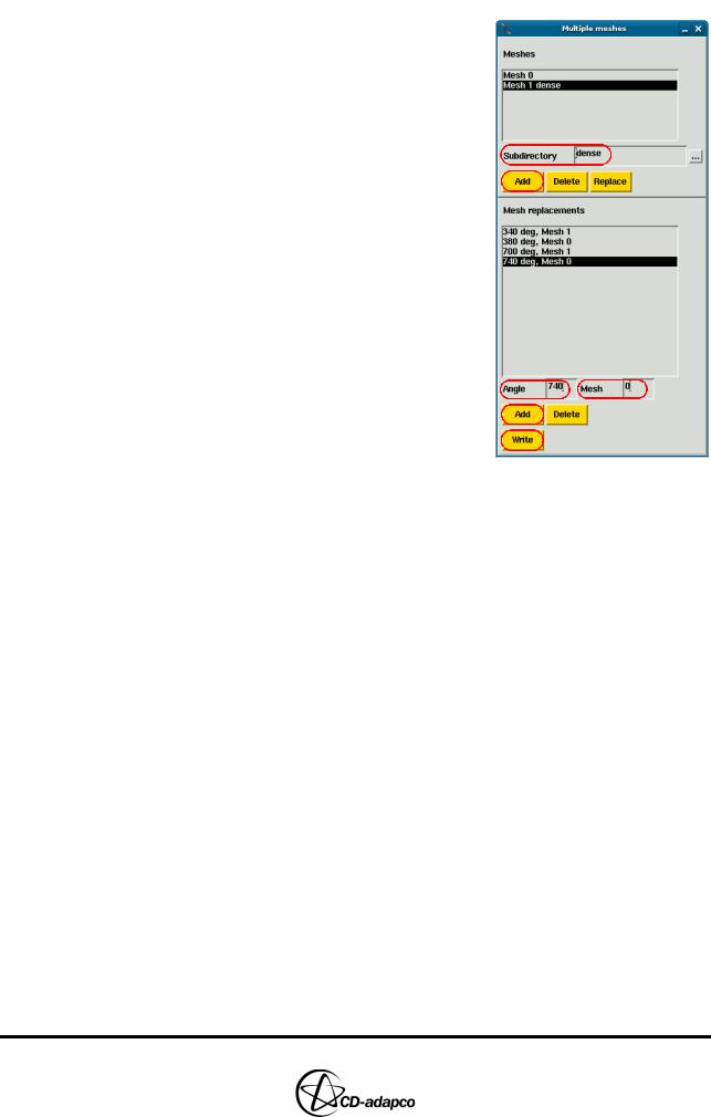
In the Select panel, click Multiple Meshes to |
||
|
open the Multiple meshes panel |
||
• |
Click the ellipsis (...) button next to the |
||
|
Subdirectory box |
|
|
• |
In the file browser, select dense and then |
||
|
click OK to specify the directory where the |
||
|
replacement mesh is located |
||
• |
Click Add in the upper half of the panel to |
||
|
specify the dense mesh in the Meshes box |
||
• |
Set Angle to 340 and Mesh to 1 to specify the |
||
|
crank angle and mesh for the first mesh |
||
|
replacement |
|
|
• |
Click Add in the lower half of the panel to |
||
|
enable the first mesh replacement |
||
• |
Define the remaining mesh replacements |
||
|
using the following settings: |
||
|
|
|
|
|
Angle |
Mesh |
|
|
|
|
|
|
380 |
0 |
|
|
|
|
|
|
700 |
1 |
|
|
|
|
|
|
740 |
0 |
|
|
|
|
|
•Click Write to create the MULTIMESH.BAT batch file and merge the mvmesh.sh files of both models into a single file. A backup of the original mvmesh.sh is created called mvmesh.sh.original.
The set-up within the coarse model is now complete.
•In the Select panel, click Write Data
•In the Write Tool, enter save_es-ice.coarse and click Save
•Close es-ice
Setting Up Mesh Replacement in pro-STAR
The pro-STAR set-up for a mesh-replacement simulation is slightly different from a normal simulation as two or more models are defined simultaneously. You must therefore ensure that the pro-STAR set-up in your own cases adheres to the following guidelines:
•The initial and boundary conditions, combustion models and any tracers defined within the es-ice Star Controls panel must be identical to the settings in pro-STAR
•Additional physics settings defined within pro-STAR are read from the problem file present in the working directory. These include settings for thermophysical, spray and/or liquid film models. In this example, both the coarse and dense model files have been set up correctly.
•Analysis and run-time controls in the model files do not need to be identical. These settings include under-relaxation, time-step size, residual tolerances, output frequency and backup frequency. In this example, the time-step
Version 4.20 |
13-9 |
controls remain as specified in es-ice but other common settings are applied to the analysis output controls for both models. The under-relaxation for pressure correction is set to 0.5.
To read the es-ice model files:
•Launch pro-STAR from the directory containing the master model file (save_es-ice.4-final)
•Enter the command below (it may take some time to complete):
IFILE, MULTIMESH.BAT
This command resizes pro-STAR memory, imports the models and creates an events file.
•Enter the following commands to display the coarse mesh:
CSET, ALL CPLOT
Setting up the coarse model
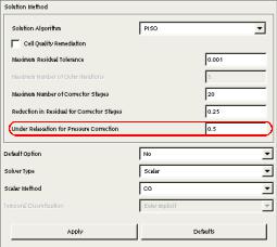
Set the under-relaxation factor as shown in Figure 13-7.
•In the Analysis Controls > Solution Method panel, set Under Relaxation for Pressure Correction to 0.5
•Click Apply
Figure 13-7 Under-relaxation for pressure correction
Specify the output control settings as shown in Figure 13-8.
•Go to panel Analysis Controls > Analysis Output
•In the Post tab, set Output Frequency to 10 and Backup Frequency to 300
•Click Apply
•In the Transient tab, set Start at time to 320 degrees CA and Output interval to
5 degrees CA
•Select any flow variables that you wish to post-process
•Click Apply
Chapter 13 |
MESH REPLACEMENT |
|
Setting Up Mesh Replacement in pro-STAR |
|
|
Figure 13-8 Post and transient analysis output settings
Setting up the dense model
Reading the MULTIMESH.BAT file into pro-STAR defines the dense model location.
•Enter the following command to switch to the dense model:
MREPLACE, SWITCH, 1
•Enter the following commands to display the dense model:
CSET, ALL
CPLOT
The parameter that is set to 1 in the previous command selects the dense model. If you wish to switch back, the coarse model can be selected using 0 as the parameter value.
Having switched to the dense model, the same settings are now used for under-relaxation and output controls. The previous panels can be used again to verify these operations.
Set the under-relaxation factor.
•In the Analysis Controls > Solution Method panel, set Under Relaxation for Pressure Correction to 0.5
•Click Apply
Version 4.20 |
13-11 |
Specify the output control settings.
•Go to panel Analysis Controls > Analysis Output
•In the Post tab, set Output Frequency to 10 and Backup Frequency to 300
•Click Apply
•In the Transient tab, set Starting at time to 320 degrees CA and Output interval to 5 degrees CA
•Select any flow variables that you wish to post-process
•Click Apply
When the pro-STAR set-up is complete, write the geometry and problem files for both models. This action creates .ccmg and .prob files in the relevant directories for both.
•Enter the following commands:
MREPLACE, GEOMWRITE, 0.001, CCM
MREPLACE, PROBLEMWRITE
The pro-STAR set-up is now complete, so:
•Click Quit > Save & Quit to close pro-STAR
The solver can now be run in the usual manner, as described in Chapter 8 of this volume.