Chapter 20 MESHING WITH THE MAPPING METHOD

The model at the beginning of this chapter can be resumed from file: save_es-ice.1-valves (created in Chapter 3)

The following tutorial data files are used in this chapter:

MAPPING_TUTORIALS/vlift01.dat

(valve lift file for Valve 1)

MAPPING_TUTORIALS/vlift02.dat

(valve lift file for Valve 2)

MAPPING_TUTORIALS/exhaust.dbs

exhaust port mesh from pro-STAR’s AutoMesh module)

The model in this chapter is intermittently saved to files: save_es-ice.2-template save_es-ice.3-flat save_es-ice.4-starsetup

An es-ice mesh can be generated using the Trimming method or the original Mapping method. The latter involves mapping of surface vertices to shells of the geometry through the use of edges, splines and patches and is covered in this chapter. The Trimming method is covered in Chapter 4.

The meshing process using the Mapping method can be divided into five major steps:

1.Creating the 2D base template

2.Creating the 3D template

3.Creating edges, splines and patches based on geometrical features

4.Mapping the 3D template surface to the geometry

5.Meshing the piston

Creating the Stub Surface in the Geometry

es-ice gives you the option of creating a mesh for arms externally, via a software package such as the AutoMesh version of pro-STAR. The externally-created arms may then be read into es-ice and matched with the rest of the model via a coupled-cell interface. Typically, this interface is shaped like a stair step and is called a “stub”. For this tutorial example, the exhaust port above Valve 2 will be meshed using pro-STAR’s AutoMesh module. As a result, a stub surface must first be created in the geometry to serve as an interface between the es-ice and pro-STAR meshes.

We create a stub shell surface by first creating splines that define the corners of the shell surface. We then create shells that span across the splines and define the surface. Usually, four splines are needed for this. Two of them will be created on the geometry surface and the other two inside the geometry. A detailed description of how to create a stub can be found in Chapter 3, “Generating the stub geometry” of the User Guide volume. The large cross-hair arrow will help to create all splines accurately at the same θ position (see Figure 20-1).

Begin by isolating Valve 2 and inspecting the valve stem. The mesh above the stub is assumed to be static, hence it is important to find a vertex on a lower section of the valve stem, above which the stem radius is constant, and create a circular spline there. To do this:

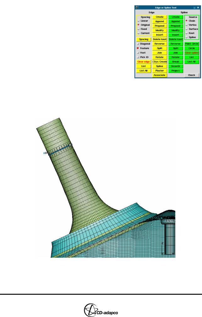
•Click Edge or Spline in the Select panel

•In the Edge or Spline Tool panel that now appears, click Point Circle

•Left-click with the mouse on a vertex to create a circular spline with the next highest available ID number (see Figure 20-1). This operation uses the nearest

cylindrical coordinate system, which will be the local coordinate system for Valve 2.

•Type q with the cursor inside the window or click on an empty part of the window to quit the ‘pick’ mode and accept the spline. Since there are no other existing splines, the created spline has an ID of 1.

Figure 20-1 Geometry window: Circular spline created around Valve 2

•In anticipation of future events, renumber this first spline so that it has an ID of 51 using the following command:

spline,1,renumber,51

All future splines will be created with larger ID numbers, thus leaving the lower ID numbers free for default splines to be employed later on.

Next, isolate the valve seat and port arm areas for the exhaust side and inspect the shells between them. Find a vertex on the highest machined point of the valve seat shells, such that it is as close as possible to the circumferential position of the previously used valve stem vertex (this will help reduce the skewness in the stub’s geometry shells when they are created later). The large cross-hair will be helpful in this process.

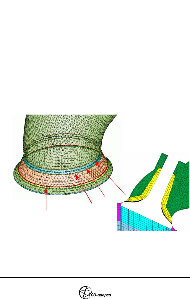
• As for the previously created spline, click Point Circle in the Edge or Spline Tool panel and left-click on a vertex to create another concentric spline (see Figure 20-2). This figure shows three possible locations where you can create the next spline. These locations will give a near-perfect circular shape. In this tutorial, we choose location #1 as indicated in Figure 20-2. The resulting map mesh is shown in the same Figure, at the location where the stub has been coupled with the polyhedral mesh of the exhaust port.

• Type q with the cursor in the window or click on an empty part of the window to accept the spline.

3

Valve Seat

Figure 20-2 Geometry window: Circular spline around the valve seat and port

The previous two splines were created on the surface geometry. Two more splines need to be created inside the model. For this you need to view all the geometry shells in a section passing through the exhaust valve centreline. Since the local coordinate system of the exhaust valve has been defined already (see Chapter 3, “Modelling the Valves” in this volume) you can use the training panel to view the

geometry shells in a section, by clicking the valve 2 section button. Make sure that the geometry shells of the exhaust valve and port are in the current cset.

You can take measurements in the local valve coordinate system from the section plot using command:

sxyz,12,relative

This command will give relative distances between successively selected points in coordinate system 12. These distances are what will be used to create the final two splines for the stub.

One spline will be created radially outwards from the first spline created on the valve stem, such that there is room for at least a few cells in the radial direction in both the stub and the externally generated mesh. The other spline will be created below it and slightly further out radially such that

(a)it is not too close to the valve surface, and

(b)the two flat surfaces connected to this spline are approximately parallel with the top surface of the valve and with the lower portion of the valve stem.

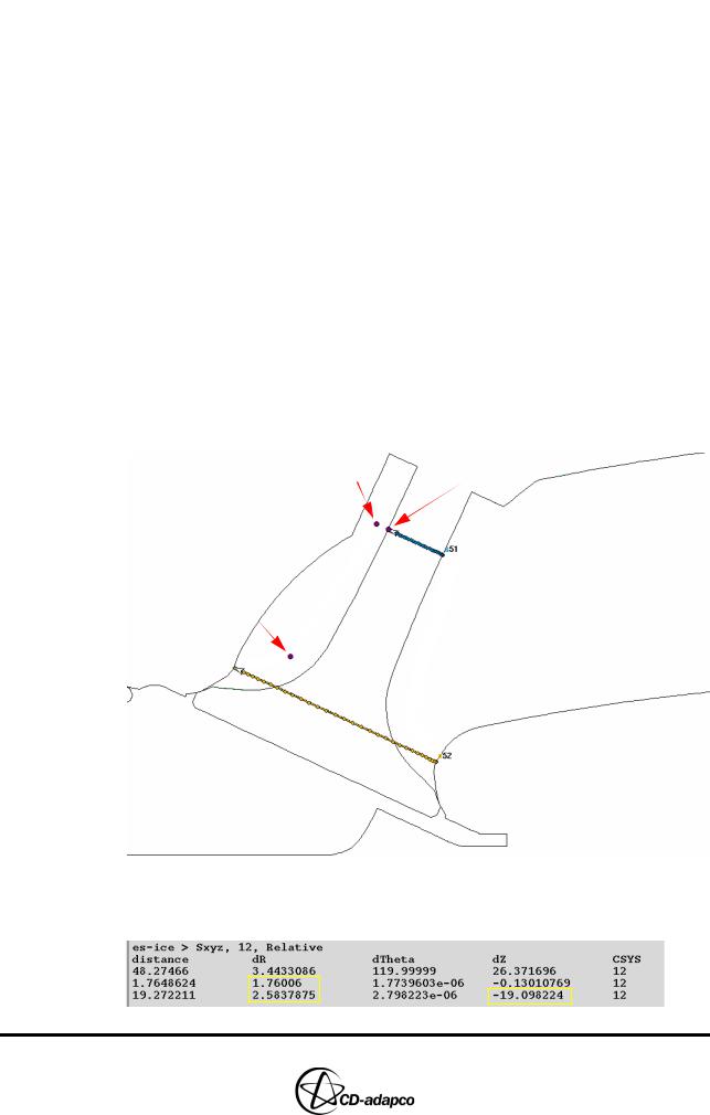
•Click on approximately the three points shown in Figure 20-3 and then type q with the cursor in the window to quit this operation.

3

Figure 20-3 Geometry window: Points picked during the sxyz command

The text output in the es-ice window should be similar to that shown below:

The first line shows the relative distances from the origin of coordinate system 12

to the first point, which approximately represents a point on the spline created on the valve stem. This can be ignored. The second line shows the relative distances from the first point to the second point. We will be using the approximate relative radial distance to create one of the splines. The third line shows the relative distances from the second point to the third point. We will be using the approximate relative radial and axial distances to create the other spline.

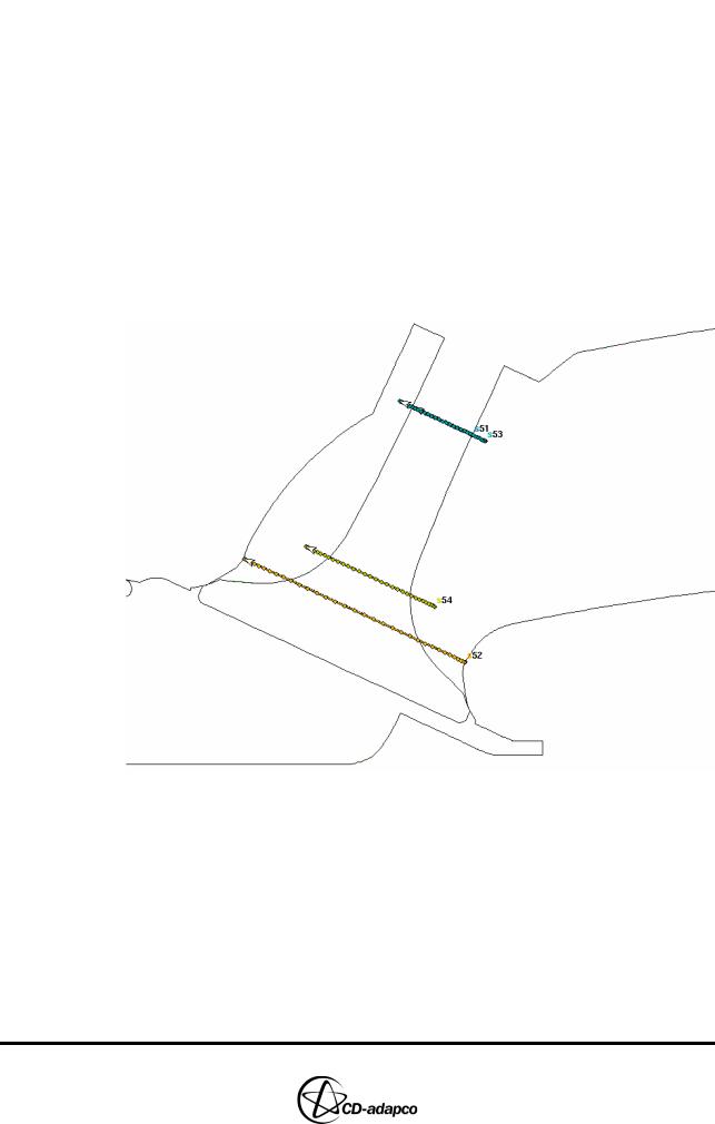
•Type the following commands to create spline 53 radially outwards from spline 51 and then create spline 54 radially outwards and axially downwards from spline 53:

spline,51,to,53,1.8,0,0,12 spline,53,to,54,2.6,0,-19,12

The four splines needed to create the stub shell surface are shown in Figure 20-4.

Figure 20-4 Geometry window: All four splines created for the stub surface

•Return to a hidden view, select an isometric viewing angle and delete all cells from the current cell set in order to be able to see the effect of subsequent commands.

•Create a layer of shells with cell type 22 between each pair of splines that represents the stub surface:

sshell,Cursor,1,22

•Select spline nos. 51 and 53 to generate the first section of the stub.

•Repeat the above steps for the other two sections of the stub: section 2 (spline

nos. 53 and 54) and section 3 (spline nos. 54 and 52).

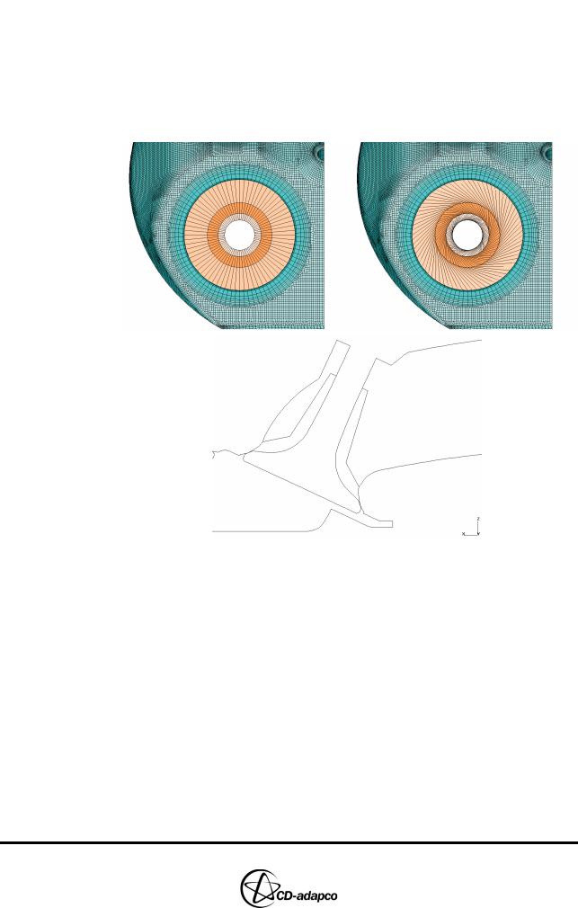
Plots of a correct and incorrect stub surface are shown in Figure 20-5. These plots emphasize the importance of making the splines start at the same θ position. This is also important for mapping edges with the splines, as will be seen later. Chapter 3, “Generating the stub geometry” in the User Guide provides more detailed information on how to generate an ideal stub geometry.

Figure 20-5 Geometry window: Correct stub (top left), incorrect stub (top right) and section (bottom) of stub surface

The necessary cells can now be exported to a database file so that pro-STAR’s AutoMesh module can be used to mesh them.

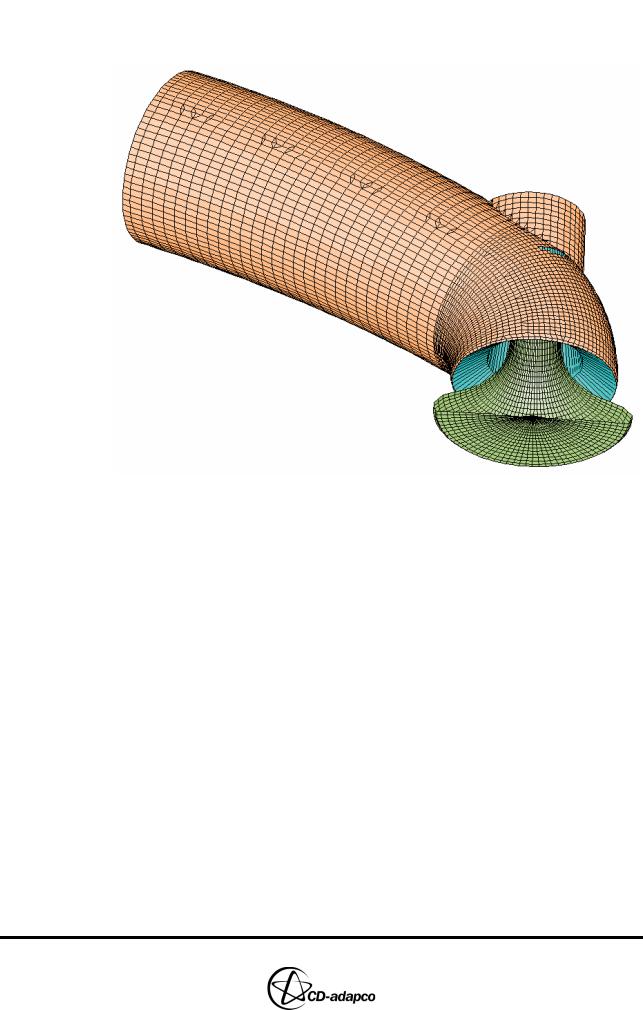
•Gather the stub, exhaust valve and port into the currently active cell set and remove all splines from the currently active spline set, see Figure 20-6.

•Click Read Data in the Select panel to open the Read Tool panel

•Type the file name, exhaust-proam.dbs, into the input field next to the Dbase button and deactivate the Exists button since this will be a new file.

•Click the Dbase button to open a new database file called exhaust-proam.dbs

•Type the following commands to store the cells and vertices in the currently

active cell set under database ID 1 as a surface definition entitled Exhaust valve+port+stub and close the database file:

dbase,put,1,surface

Exhaust valve+port+stub dbase,close

Figure 20-6 Selected geometry to be exported to exhaust-proam.dbs

Now this database file may be used by the AutoMesh module to generate the necessary mesh. For the purposes of this tutorial example, the exhaust port mesh is assumed to have been created already in file exhaust.dbs along with the other tutorial example files.