


3.4 Developing the Model |
29 |
of risk analysis in investment costs management is described, based on the example of the project of the Waste Treatment Facility using pyrolysis method with energy recovery for the City of Konin and Konin district (Oferta 2002). The Waste Treatment Facility was supposed to be built based on American technology introduced by a consortium of the following companies: IESSCO Inc., NORCON INTERNATIONAL Inc., SIMONDS MFG. Corp., BECO ENGINEERING Co., CP. Mfg. Inc., MARATHON EQUIP. Inc., and FOSSIL ENERGY GOV. The facility was set to include two complete units, responsible for the pyrolysis and gasification of municipal waste, with a daily output of 200 metric tons of waste.
3.4Developing the Model
The six stages of the Waste Treatment Facility Project as well as the total value of the projected investments costs (TOTAL – see Table 3.1) have been taken into consideration during the analysis. The simulation has been conducted using Simlab® software – a simulation package that is equipped with features such as: full visualisation of the performed simulation and clear methods for inputting data and recording obtained results. In addition, Simlab® offers a range of distribution types (normal, log-normal, uniform, etc.).
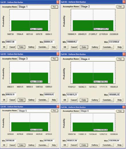
The specification of investment costs is shown in Table 3.1. The values are given in US Dollars (USD), since the presented offer was originally drawn up based on that currency. In this thesis, it is established that random cost values of the investment, in its individual stages, may be described using uniform distribution, based on the work of Liberman (2003) who, in his economic analysis of the
Table 3.1 The projected investment costs, based on the American project (values shown in USD), along with parameters of uniform distribution
City of Konin
The Waste Treatment Facility project
|
Investment stages |
Partial cost |
a – lower |
b – higher |
|
|
(in USD) |
interval value |
interval value |
|
|
|
|
|
1 |
Stage 1 – management, investment, design, |
600731.00 |
540657.90 |
660804.10 |
|
permissions |
|
|
|
2 |
Stage 2 – the waste gasification facility building, |
21120055.27 |
19008049.70 |
23232060.80 |
|
gasification facility (boilers, transport, |
|
|
|
|
permissions, assembly) |
|
|
|
3 |
Stage 3 – monitoring of gas emission |
999599.10 |
899639.19 |
1099559.01 |
4 |
Stage 4 – conveyor belts, automatic loading |
1687350.23 |
1518615.21 |
1856085.25 |
|
system, design supervision, engineering, |
|
|
|
|
start-up |
|
|
|
5 |
Stage 5 – office equipment, computers, transport |
425000.00 |
382500.00 |
467500.00 |
|
facilities, lifts, etc. |
|
|
|
6 |
Stage 6 – investment reserve |
1167264.40 |
1050537.96 |
1283990.84 |
|
Total cost – TOTAL |
26000000.00 |
|
|
30 |
3 The Role of Risk Assessment in Investment Costs Management |
Fig. 3.1 Graphical presentation of the density function of random input parameters of model approximation using uniform distribution, in Crystal Ball software (Source: Own work)
construction of wind power plants in the United States, has used uniform distribution in the approximation of random cost values in the investment’s budget. As is argued by Snopkowski (2007), uniform distribution, despite its limited capabilities in terms of modelling of real processes, has a wide range of applications in stochastic simulation algorithms. Interval values [a, b] of uniform distributions, estimating the random cost values of the investment (Stage 1–Stage 6), can be found in Table 3.1. The values of a and b are calculated on the basis of automatic estimation using CB, following the steps given in Chap. 2 (see Chap. 2). Mean values (Fig. 3.1) are equivalent to deterministic costs of separate investment stages presented in Table 3.1.
3.4 Developing the Model |
31 |
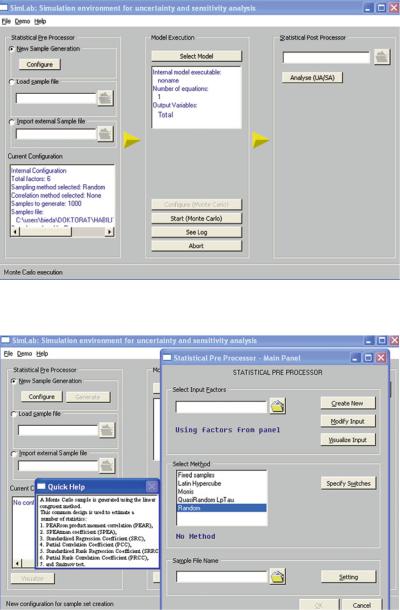
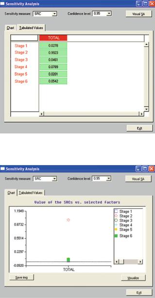
Fig. 3.2 The main screen of the Simlab® program
Fig. 3.3 Main Panel window
The main screen of the Simlab® program is shown in Fig. 3.2. The construction of the model can be started by clicking on the Configure button, seen on the main screen of the program (Fig. 3.2). Once clicked, a new window appears (Main Panel), as presented in Fig. 3.3. After clicking on the Create New button, another
32 |
3 The Role of Risk Assessment in Investment Costs Management |
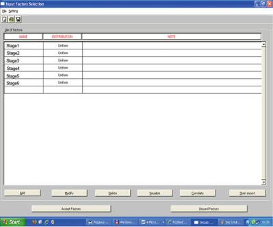
Fig. 3.4 Input Factors Selection window
window appears (Input Factors section), a representation of which can be seen in Fig. 3.4, which serves as a tool for creating distributions estimating input parameters of the model.
3.5Defining Input Data: Organising the Simulation
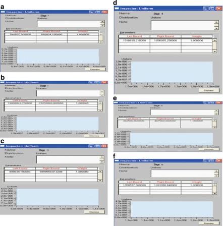
Before running the simulation, the input data, received in the graphic form presented in Fig. 3.5 (a–f) (Bieda 2010), is defined.
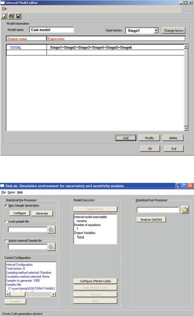
The model constituting the total cost – TOTAL, characteristic due to its six stages (Stage 1–Stage 6), is shown in Fig. 3.6.
3.6Activating the Model: The Results of the Simulation
In order to start a model it is required to first use the Random option, which can be selected from the Main Panel window (Fig. 3.3) that serves as a starting point for MC simulation. After choosing the Random option, a new Quick Help window appears to the left of the Select Method dialog box, which informs us about the
3.6 Activating the Model: The Results of the Simulation |
33 |
Fig. 3.5 Graphical presentation of the density function of random input parameters of model approximation using uniform distribution, in SimLab software (Source: Own work)
availability of possible data analysis methods based on randomness. The Specify Switches button takes us to a new window, which is used to specify different parameters of the simulation (such as the number of randomisation steps). By clicking on the Configure (Monte Carlo) button (Fig. 3.7) and then in turn on the Select Model and Start (Monte Carlo), as is shown in Fig. 3.8, Monte Carlo simulation begins to run. The results of the simulation can be presented in the form of sensitivity analysis (SA) and uncertainty analysis (UA) by clicking on the Analyse (UA/SA) button (Fig. 3.8) and by clicking on the UA or SA button, available from the Statistical Post Processor – Main Panel window (Fig. 3.9), launched automatically once the abovementioned Analyse (UA/SA) button is activated. Sensitivity analysis with the confidence level of 95%, created on the basis of Spearman Rank Correlation coefficients (SCR), for the data presented in Table 3.1, is shown in Figs. 3.10 and 3.11. In Fig. 3.11 the chart’s vertical axis is
34 |
3 The Role of Risk Assessment in Investment Costs Management |
Fig. 3.6 Internal Model editor window (Source: Own work)
Fig. 3.7 The sensitivity and uncertainty analysis window: Monte Carlo configuration
3.6 Activating the Model: The Results of the Simulation |
35 |
Fig. 3.8 The sensitivity and uncertainty analysis window: Start Monte Carlo
Fig. 3.9 Statistical Post Processor – Main Panel window with a list of uncertainty (UA) and sensitivity analysis (SA) buttons (Source: Own work)
36 |
3 The Role of Risk Assessment in Investment Costs Management |
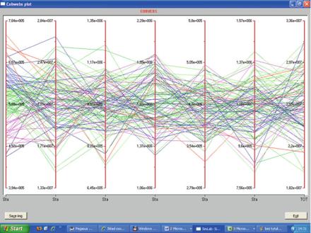
Fig. 3.10 Sensitivity analysis with confidence levels of 95% (SRC – Spearman Rank Correlation) – tabular form (Source: Own work)
Fig. 3.11 Sensitivity analysis with confidence levels of 95% (SRC – Spearman Rank Correlation) – dot diagram (Source: Own work)
scaled according to the values of Spearman Rank Correlation coefficients, but at the same time it is worth remembering that the rank correlation coefficient’s values are within the specified range of [ 1; 1]. It can be concluded, from the analysis of
3.6 Activating the Model: The Results of the Simulation |
37 |
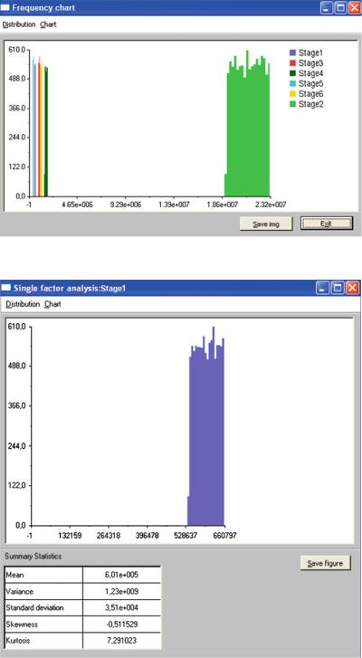
Fig. 3.12 Cobwebs plot sensitivity analysis under confidence levels of 95% (SRC – Spearman Rank Correlation) (Source: Own work)
the chart that the key variable, which influences the total cost of the project the most, is Stage 2 (correlation coefficient ¼ 0.9923). The positive sign of the coefficient signifies the existence of positive correlation, whereas the negative sign marks negative correlation. While evaluating the results it is important to draw one’s attention to whether correct requirements have been met regarding the number of randomisation steps in the cycle. The green colour of cells in the TOTAL column, containing the values of Spearman Rank Correlation coefficients, means the randomisation has been performed correctly. A flawed randomisation (too few steps) generates results, which are inserted in the TOTAL column cells and are coloured red (Saltelli et al. 2004).
The instruction – Visual SA – allows the user to present the simulation results in a graphic form. An example of a visualisation in the form of the Cobwebs plot can be seen in Fig. 3.12. This graph helps us better understand the state of the model’s certain parameters, while the simulation process is underway. In Fig. 3.12, the chart’s horizontal axis is labelled with both the symbols of different stages (1–6) that appear in the cost model, and the symbol of total cost – TOTAL. The range of confidence intervals can be read from the frequency charts, shown in Figs. 3.13–3.19, built as a result of uncertainty analysis performed using MC simulation.
38 |
3 The Role of Risk Assessment in Investment Costs Management |
Fig. 3.13 Uncertainty analysis frequency chart – cumulative, of all six stages (Source: Own work)
Fig. 3.14 Uncertainty analysis frequency chart – Stage 1 (Source: Own work)
3.6 Activating the Model: The Results of the Simulation |
39 |
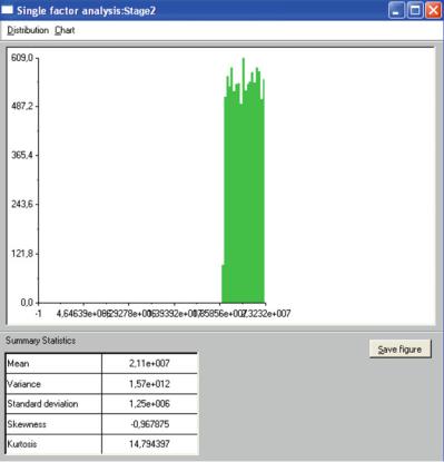
Fig. 3.15 Uncertainty analysis frequency chart – Stage 2 (Source: Own work)
The results of the uncertainty analysis, obtained after using the UA button (Fig. 3.8), are shown in Figs. 3.20 and 3.21 in the form of frequency charts (confidence level of 95%). The frequency chart along with the statistic report, received after the activation of the TOTAL field (a square in the top right hand corner of the chart (Fig. 3.21)) is presented in Fig. 3.21. Both figures display a horizontal axis, which is labelled with the total investment cost values TOTAL (shown in USD). The mean value, which is equal to 2.6E + 7, is equivalent to the deterministic total cost of the investment – TOTAL (Table 3.1). It can be observed, by analysing Table 3.2 that, starting from zero, the higher the frequency (the second column) the higher the increment (the third column). The read value of x ¼ TOTAL equals 2.45E + 7. When frequency reaches the value of 614, which is equivalent to the value of x ¼ 2.1E + 7, its value begins to fall, until it reaches zero (its increment falls and gets close to zero as well), while its corresponding value is
40 |
3 The Role of Risk Assessment in Investment Costs Management |
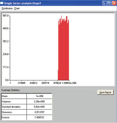
Fig. 3.16 Uncertainty analysis frequency chart – Stage 3 (Source: Own work)
x ¼ 2.98E + 7. Thus, it can be noted that the obtained confidence interval is described with the values of [2.454E + 7; 2.98E + 7] (shown in USD), and its span can be expressed by the number 5.3E + 6.
The total (deterministic) value of investment costs, presented in the row ‘Total’ in the Table 3.1, amounts to 2.6E + 7 USD. In the stochastic approach to design, however, the mean random value of the total investment costs, worked out as a result of the simulation, amounts to 2.73E + 7 USD. Therefore, we may be 95% confident that the confidence interval covers the mean value of the total investment costs, or in other words, the mean value of the total investment costs is between the number 2.45E + 7 USD and the number 2.98E + 7 USD, with the same 95% confidence level.