

2.4 The Results of the Simulation |
17 |
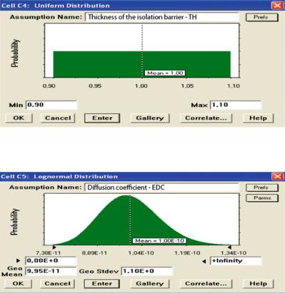
Fig. 2.6 Dialog box Ð log-normal distribution for the thickness of isolation barrier variable Ð TH (Source: Own work)
Fig. 2.7 Dialog box Ð log-normal distribution for the diffusion coefÞcient variable Ð EDC (Source: Own work)
2.4The Results of the Simulation
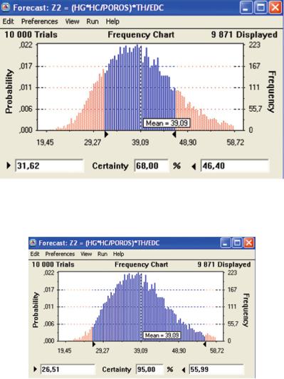
After activating the simulation, according to the algorithm (2.1) (having previously set the randomisation cycle, which, in the analysed case, has 10000 trials), the numerical results of the Z2 forecast calculations are presented in the form of frequency charts (Figs. 2.8, 2.9) and statistic reports (Figs. 2.10, 2.11). The results of MC simulation with different conÞdence levels are shown in Figs. 2.8 and 2.9. In the uncertainty analysis connected to LCA methodology, the 68% conÞdence levels are used quite frequently (Sonnemann et al. 2004; Rabl and Spadaro 1999; Spadaro and Rabl 2008). In the Forecast window, one can notice a frequency chart along with some tools that modify it. These modiÞers, or grabbers, presented in the form of small black triangles, indicate where, after a Þnished simulation, is the right and left end of the conÞdence interval. In the frequency chart (Figs. 2.8 and 2.9) the conÞdence interval span is highlighted with a darker colour marker (the probability
18 |
2 Stochastic Model of the Diffusion of Pollutants in LandÞll Management |
Fig. 2.8 Frequency chart of the Z2 forecast expression (68% conÞdence level) (Source: Own work)
Fig. 2.9 Frequency chart of the Z2 forecast expression (95% conÞdence level) (Source: Own work)
that X assumes the values in the conÞdence interval, is equal to the measure of the cell under the darker part of the frequency chart). By writing: Z2 ¼ (HG*HC/ POROS)*TH/EDC in the Certainty edit Þeld of the Forecast dialog box, and by
2.4 The Results of the Simulation |
19 |
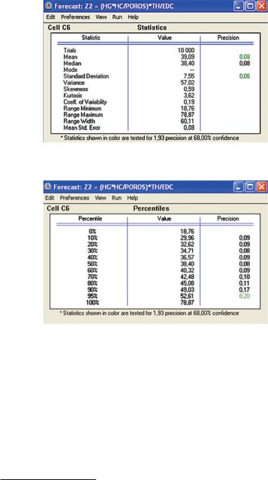
Fig. 2.10 Statistical report of the Z2 expression forecast Ð Statistics
Fig. 2.11 Statistical report of the Z2 expression forecast Ð Percentiles (Source: Own work)
setting the values to 68% and 95%, respectively,5 the span of the conÞdence intervals is set automatically by the grabbers, and the corresponding numerical values are entered in the edit Þelds in the bottom part of the dialog boxes of the Forecast tab: Z2 ¼ (HG*HC/POROS)*TH/EDC.
ConÞdence interval, theoretical basis of which was postulated in 1993 by a Polish statistician, J. Spława-Neyman, deÞnes the probable scope of calculation deviation from the real value (Stanisz 2006). In other words, the simulation results provide an opportunity to realise the span of the random conÞdence intervals that will cover the estimated values of the Z2 forecast. Additionally, the author wishes
5 The 68% conÞdence interval is synonymous to an interval equivalent of the 68% conÞdence level.
20 |
2 Stochastic Model of the Diffusion of Pollutants in LandÞll Management |
to present, for comparison purposes, the results of uncertainty analysis for the 95% conÞdence level, which is quoted in the literature as being the ÒclassicÓ amount (Tadeusiewicz 1999). The 95% conÞdence levelÕs recommendation can be found, among others, in the Eco-indicator method (Eco-indicator 99 2009) and in the Regulation of the Minister of Environment of 12 September 2008 on the means of monitoring emission levels of substances covered by the emission allowance trading scheme of the Community (D.U. 2008). As a result of the carried out simulation, the conÞdence intervals, equivalent to the 68th and 95th percentage level of conÞdence, are equal to [31,62; 46,40] and [26,51; 55,99], respectively (Figs. 2.8, 2.9).
2.4.1Sensitivity Analysis
Sensitivity analysis of input data is extremely useful both in environmental testing and in investment processes. In the subject literature, one can encounter different versions of its deÞnition (de Koning et al. 2010) and it is perceived, by some sources, as the most important outcome of MC simulations using CB software (Bradly 1999; Gaudet 1997; Lorance and Wendling 1999; Warith et al. 1999; Yenni 1999; Saltelli et al. 2004, 2008). The method indicates which input parameter of a model is of greatest inßuence on the Þnal result of the simulation, or, in other words, it demonstrates the usefulness of particular critical variables, i.e. the ones that signiÞcantly inßuence the value of an expression. Depending on the choice in the drop-down menu in the Sensitivity Chart tab and the View command, the diagram will be created by comparing SpearmanÕs rank correlation coefÞcients, sorted in descending order, where positive correlation coefÞcients indicate that the acceptance of the stricter assumptions can be associated with obtaining the higher forecast probability. On the other hand, negative correlation coefÞcients point to an opposite tendency, or the measured contribution of the modelÕs entry variables on variance, or to put it differently, the deÞnition of the involvement, of critical variables in the model, in the variation of the dependent variableÕs mean value (the Z2 expression). Evans and Olson (1998), by brießy outlining the problems associated with MC simulation, have formulated a statement that correlation coefÞcients combine hypotheses with forecasts. Suh and Rousseaux (2002) have used sensitivity analysis in LCA studies, the aim of which is to compare the environmental impact of Þve sludge management methods in France (see Kowalski et al. 2007). The graphic presentation of sensitivity analysis is most effective when, at most, 10 (ten) parameters are analysed; if there are more, it becomes unpractical (Uncertainty 2008).
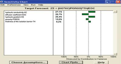
Crystal Ball has integrated statistical, optimisation, and prognostic tools; this results in the elimination of both the uncertainty element and the lack of conÞdence in the deterministic values of parameters that form the Z2 expression (Bieda 2002). The sensitivity analysis shown in Fig. 2.12 suggests that hydraulic conductivity (HC) has the most signiÞcant inßuence on the variability of the Z2 expression.
2.4 The Results of the Simulation |
21 |
Fig. 2.12 Sensitivity analysis of the Z2 expression forecast (Source: Own work)
Hydraulic gradient (HG) as well as the thickness of the isolation barrier (TH) are next in line. Their respective variance share is: 27.1%, 26.4%, and 9.2%. When it comes to diffusion coefÞcient (EDC) and porosity (POROS), however, their inßuence is negative and amounts to 26.7% and 10.6%, respectively (Li and Wu 1999).
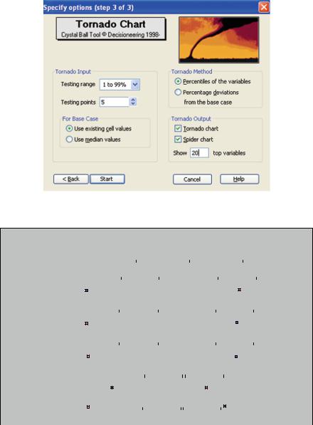
The recommended method of the modelÕs analysis of its sensitivity to the change of value of individual variables is the graphic method of evaluating the analysed modelÕs sensitivity to individual variables, for the speciÞed type of distribution. Crystal Ball offers the ability to generate tornado charts and spider charts. In order to create the abovementioned charts, the Tornado Chart option needs to be picked from the drop-down CB Tools menu, which can be found on the main menu bar of the CB program. The Specify Options dialog box, in the third step (Fig. 2.13), allows the user to enter individual quantities, characteristic of the creation of tornado and spider charts. The following elements are used in this process: input data (Tornado Input), the method of creating the chart (Tornado Method), the type of input data used to create the chart (Use existing cell values), and the types of charts (Tornado Output). After making the choice, the program runs the procedure of constructing sensitivity analysis in the form of a tornado and/or a spider chart. The outcome of the analysis in the form of a tornado chart is shown in Fig. 2.14. This diagram has been constructed on the basis of data included in the sensitivity Table 2.2. The values of the impact of the analysed variables on the value of the Z2 expression (forecast) is presented in the form of horizontal bars, bearing in mind that the most crucial ones are at the top of the chart and the less important ones at the bottom. Next to each bar there is a calculated value of the parameters within the upper and lower interval ranges for the deÞned probability distribution. The error bars indicate standard errors.
An alternative way of presenting output data is the use of line graphs, also known as spider charts. These have Þve series of data containing reporting for individual input variables of the Z2 value. The horizontal x-axis maps the location measure of
22 |
2 Stochastic Model of the Diffusion of Pollutants in LandÞll Management |
Fig. 2.13 The Tornado Chart dialog box with the options to create tornado and spider charts
Z2 = (HG*HC/POROS)*TH/EDC
2.00E+01 |
|
|
|
3.00E+01 |
4.00E+01 |
|
|
|
5.00E+01 |
6.00E+01 |
|||||||||
Diffusion coefficient - |
|
|
|
|
|
|
|
|
|
|
|
|
|
|
|
|
|
|
|
|
|
|
|
|
|
|
|
|
|
|
|
|
|
|
|
|
|
|
|
|
|
|
|
|
|
|
|
|
|
|
|
|
|
|
|
|
|
|
|
EDC |
|
|
|
|
|
|
|
|
|
|
|
|
|
|
|
|
|
|
|
|
|
Upper boundary; diffusion |
|
|
|
|
|
|
|
Lower boundary; diffusion |
|
|
|
||||||
Hydraulic conductivity - |
|
coefficient-EDC: 3.07E+01 |
|
|
|
|
|
|
|
coefficient-EDC: 4.89E+01 |
|
|
|||||||
|
|
|
|
|
|
|
|
|
|
|
|
|
|
|
|
|
|
|
|
|
|
|
|
|
|
|
|
|
|
|
|
|
|
|
|
|
|
|
|
HC |
|
|
|
|
|
|
|
|
|
|
|
|
|
|
|
|
|
|
|
|
|
Lower boundary; hydraulic |
|
|
|
|
|
|
|
Upper boundary; hydraulic |
|
|
|
||||||
Hydraulic gradient - |
|
conductivity-HC: 3.04E+01 |
|
|
|
|
|
|
|
conductivity-HC: 4.84E+01 |
|
|
|||||||
|
|
|
|
|
|
|
|
|
|
|
|
|
|
|
|
|
|
|
|
|
|
|
|
|
|
|
|
|
|
|
|
|
|
|
|
|
|
|
|
HG |
|
|
|
|
|
|
|
|
|
|
|
|
|
|
|
|
|
|
|
|
|
Lower boundary; hydraulic |
|
|
|
|
|
|
|
Upper boundary; hydraulic |
|
|
|||||||
Porosity - POROS |
|
gradient-HG: 3.04E+01 |
|
|
|
|
|
|
|
gradient-HG: 4.84E+01 |
|
|
|
||||||
|
|
|
|
|
|
|
|
|
|
|
|
|
|
|
|
|
|
|
|
|
|
|
|
|
|
|
|
|
|
|
|
|
|
|
|
|
|
|
|
|
|
|
|
|
|
|
|
|
|
|
|
|
|
|
|
|
|
|
|
|
|
|
|
Upper boundary; porosity- |
|
|
Lower boundary; porosity- |
|
|
|
|
||||||||
Thickness of the |
|
|
|
|
|
POROS: 3.51E+01 |
|
|
|
POROS: 4.28E+01 |
|
|
|
|
|||||
|
|
|
|
|
|
|
|
|
|
|
|||||||||
|
|
|
|
|
|
|
|
|
|
|
|
|
|
|
|
|
|
|
|
|
|
|
|
|
|
|
|
|
|
Upper boundary; Thickness of the |
|
|
|
||||||
|
|
Lower boundary; |
|
|
|
|
|
|
|
|
|
||||||||
isolation barrier - TH |
|
Thickness of the isoloation barrier- |
|
|
|
|
|
|
|
Isolation barrier- |
|
|
|
||||||
|
|
|
TH: 3.48E+01 |
|
|
|
|
|
|
|
TH: 4.24E+01 |
|
|
|
|||||
|
|
|
|
|
|
|
|
|
|
|
|
|
|
|
|
|
|
|
|
Fig. 2.14 Tornado sensitivity chart. The error bars indicate mean standard error (Source: Own work)
distribution ranging from the 1st to the 99th percentile of data (it measures the concentration of units, as percentages). The location measures point to the placement of the value that represents the variable values in the best way possible

2.4 The Results of the Simulation |
23 |
Table 2.2 The MC simulation results, using CB software, of the sensitivity analysis of the diffusion of contaminants Ð sensitivity table (table of data) of the tornado chart
Parameter |
Z2 ¼ (HG*HC/POROS)*TH/EDC |
Input parameters |
|
||||
|
|
|
|
|
|
|
|
|
Lower |
Upper |
Range |
Min. |
Max. |
Base value |
|
|
boundary |
boundary |
|
|
|
|
|
|
|
|
|
|
|
|
|
Diffusion coefÞcient Ð |
4.89E þ 01 |
3.07E þ 01 |
1.82E þ 01 |
7.89E-11 |
1.25E-10 |
1.00E-10 |
|
EDC |
3.04E þ 01 |
4.84E þ 01 |
1.80E þ 01 |
|
|
|
|
Hydraulic conductivity |
7.89E-10 |
1.25E-09 |
1.00E-09 |
||||
Ð HC |
3.04E þ 01 |
4.84E þ 01 |
1.80E þ 01 |
|
|
|
|
Hydraulic gradient Ð HG |
1.065104692 |
1.694157822 |
1.35 |
||||
Porosity Ð POROS |
4.28E þ 01 |
3.51E þ 01 |
7.63E þ 00 |
0.3157 |
0.3843 |
0.35 |
|
Thickness of the |
3.48E þ 01 |
4.24E þ 01 |
7.56E þ 00 |
0.902 |
1.098 |
1 |
|
isolation barrier Ð |
|
|
|
|
|
|
|
TH |
|
|
|
|
|
|
|
|
|
|
|
|
|
|
|
Table 2.3 The MC simulation results, using CB software, of sensitivity analysis of the diffusion of contaminants Ð sensitivity table (table of data) of the spider chart
Parameter |
Z2 ¼ (HG*HC/POROS)*TH/EDC |
|
|||
|
1.0% |
25.5% |
50.0% |
74.5% |
99.0% |
Diffusion coefÞcient Ð EDC |
48.89 |
41.40 |
38.76 |
36.30 |
30.74 |
Hydraulic conductivity Ð HC |
30.43 |
35.94 |
38.38 |
40.99 |
48.40 |
Hydraulic gradient Ð HG |
30.43 |
35.94 |
38.38 |
40.99 |
48.40 |
Porosity-POROS |
42.76 |
40.56 |
38.57 |
36.77 |
35.13 |
Thickness of the isolation barrier Ð TH |
34.79 |
36.68 |
38.57 |
40.46 |
42.35 |
|
|
|
|
|
|
(Ostasiewicz et al. 1995; Stanisz 2006). The y-axis, on the other hand, denotes the values of Z2. These statements can be understood, statistically speaking, on the basis of porosity, as: the value of POROS reaching 99% of population is less than or equal to 35.13, the value of POROS reaching the half (50%) of population is less than or equal to 38.57, while the value of POROS reaching just 1.0% of population is less than or equal to 42.76. The graph has been constructed using the data included in Table 2.3, generated by Crystal Ball during the process of making the sensitivity analysis spider charts. The line graph is shown in Fig. 2.15. The process of performing multiple calculations of the Z2 expression value can create this type of a graph, and the value that it assumes for different tested variables, for instance, is 1%, 25%, 50%, etc., of population (i.e. the population being above or below this observation, or in other words, the set of all the measurement results that are of interest to us). It is said that, for instance, the 25th percentile divides the population into two parts resulting in a situation where 25% of population units have values no greater than the threshold value of Z2, and 75% of population units have values no smaller than the threshold value of Z2. The greater the incline of the line describing the value of the Z2 expression, the more critical the input variable becomes.