

5.6 The Analysis of the Results |
133 |
5.6The Analysis of the Results
The performed LCA analysis makes it possible to determine the environmental impact of the management of waste generated by MSP. The fact that the individual waste types are grouped and that the processes chosen from a database and used during the analysis are not adequate to Polish but to European conditions, which may generate inaccurate or even incorrect results, should be taken into consideration here.
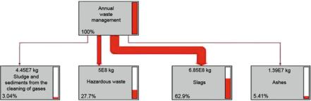
The total life cycle impact of the management of waste produced by MSP Power Plant, from an annual perspective, expressed in eco-points, amounts to 24.28 MPt (see Table 5.5 and Fig. 5.8).
The greatest potential environmental strain (approximately 63%) is caused by the storage of slag. The less straining impacts are caused by the storage of hazardous waste (27.7%) as well as coal fly-ashes and slag-ash mixtures (5.4%). The environmental impact of the remaining types of waste does not exceed 3.5%. The results of the analysis are presented in the tree form in Fig. 5.9. The tree boxes
Table 5.5 |
The LCA analysis results of the management of waste produced in the MSP Power |
||
Plant, divided into 11 impact categories |
|
|
|
|
|
|
|
No. |
Impact category |
Value [Pt] |
Share [%] |
|
|
|
|
1. |
Carcinogenic agents |
1623832.0 |
6.69 |
2. |
Respiratory system – organic compounds |
2597.8 |
0.01 |
3. |
Respiratory system – non-organic compounds |
3776919.8 |
15.55 |
4. |
Climate change |
531415.9 |
2.19 |
5. |
Radiation |
6106.6 |
0.03 |
6. |
Ozone layer depletion |
165.8 |
0.00 |
7. |
Eco-toxicity |
14528467.0 |
59.83 |
8. |
Acidification/eutrophication |
152651.7 |
0.63 |
9. |
Land use |
762692.9 |
3.14 |
10. |
Consumption of resources (minerals) |
382507.0 |
1.58 |
11. |
Fossil fuels |
2513754.0 |
10.35 |
12. |
Total |
24281111 |
100 |
|
|
|
|
Source: The Polish Academy of Sciences study (Ocena 2009)
Fig. 5.9 The simplified tree graph, concerning waste management, presenting life cycle impact of the management of waste produced by MSP. Power Plant, from an annual perspective, expressed in percentages. Source: The Polish Academy of Sciences study (Ocena 2009)
134 |
5 Stochastic Analysis, Using Monte Carlo (MC) Simulation |
detail the percentages of impact environments, which are equivalent to the values presented in brackets.
The specific values of the impact of individual categories, are presented in Table 5.5.
5.7Stochastic Analysis as an Uncertainty Calculation Tool in the LCA Study
The LCA analysis overlaps with a stochastic compound, which is an outcome of the uncertainty of data included in the Eco-indicator 99 method. Kowalski et al. (2007) describe stages of data uncertainty and their origin. Some data are based on Western European averages and are scaled towards the Eastern European ones. A degree of
5.7 Stochastic Analysis as an Uncertainty Calculation Tool in the LCA Study |
135 |
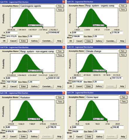
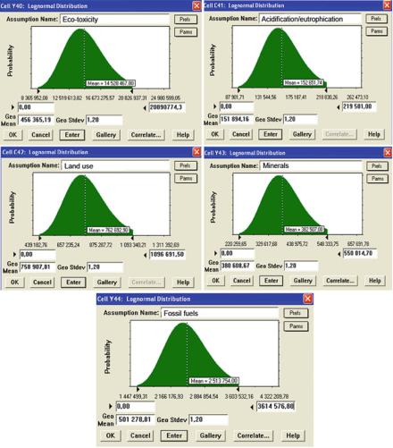
Fig. 5.10 The dialog windows of log-normal probability distribution of 11 impact categories, offered in CB software, for the LCA analysis of waste management in MSP (Source: Own work)
uncertainty, in such a situation, may reach 50% (e.g. in the case of pesticides). As uncertainty can be quite substantial and its level may be difficult to assess, it is crucial to apply different types of statistical methods, e.g. MC method. Uncertainty can be detected with relative ease through standard deviation range if appropriate statistical information is available. Even the authors of the Eco-indicator 99 methodology claim that it is not a perfect approach; nevertheless, the best possible scientific data was used in its development (Kowalski 2005). The use of all-European data (the database found in SimaPro program) may further damage the credibility of the results, as this type of data is not always adequate to Polish conditions.
136 |
5 Stochastic Analysis, Using Monte Carlo (MC) Simulation |
The LCA results, which include the sum of the 11 impact categories, presented in Table 5.5, have been used in the MC simulation. Assuming that in order to assess the impact categories different log-normal distributions may be used, in accordance with the studies cited in Chap. 4, the geometric standard deviation sg ¼ 1.2 is defined for all 11 distributions. The graphic illustration of log-normal probability distributions used to assess each of the 11 random impact categories, offered in CB software (Lognormal Distribution tab windows), are shown in Fig. 5.10. Mean values m are consistent with the deterministic values of the impact category variables (Table 5.5). With the standard geometric deviation sg, the upper boundary of log-normal distribution needs to be “adjusted” (by sliding the mini-grabbers, placed on the right-hand side of the window, accordingly), so that the mean values m correspond to the deterministic values of the impact category variables (Table 5.5). The obtained upper boundary of the distribution is then automatically entered in the edit box placed on the right in the Log-normal Distribution dialog window. The lower distribution value ¼ 0.
5.8The Results of the Simulation
The obtained simulation results, in the defined 10,000-randomisation cycle, presented in the graphic form (forecast frequency charts – Forecast: TOTAL), are shown in Figs. 5.11 and 5.12. During the simulation, different statistical data has been obtained (Statistics, Percentiles), which is shown in Figs. 5.13 and 5.14. The dialog windows – Forecast: TOTAL of the frequency charts, make it possible to assess certainty intervals. By inputting a defined value of the uncertainty level in the edit field (Certainty), Crystal Ball automatically performs the interval estimation. The confidence limits are marked with mini-sliders and their corresponding numerical values can be entered in the edit fields placed at the bottom of the Forecast: TOTAL dialog windows.
The confidence intervals corresponding to the 68th and 95th percentage point, respectively, of the confidence level of the estimated value of the total life cycle impact of the management of waste generated in an annual cycle (in 2005) are equal to, respectively:
[21596170.95; 26993165.08] Pt confidence level of 68% [19453939.35; 29587007.48] Pt confidence level of 95%
The entire range width between the left and the right edge of the frequency chart (Figs. 5.11, 5.12) is 16423946.56 Pt (Fig. 5.13); this is equivalent to the difference between the 0th and the 100th percentile, as can be seen in Fig. 5.14. The display range is between 15993187.84 Pt and 32417134.40 Pt (Fig. 5.14).