2.3 Activating the Model: Simulation

To use CB we must perform the following steps:

Step 1. The development of the simulation model using the spreadsheet function. Step 2. The deÞnition of variables, which are to become probabilistic variables.

Thus, particular variables need to be approximated with an appropriate distribution of probability.

Step 3. The selection of a spreadsheet cell, in which the forecast will be inserted. Step 4. The process of running the simulation. The maximum number of trials is

10,000 (ten thousand) (Evans and Olson 1998).

CB software has a very attractive feature that allows the user to graphically demonstrate the results of the simulation in the form of frequency charts, cumulative charts, sensitivity analyses, as well as statistic reports. The reports are presented using tables.

2.3Activating the Model: Simulation

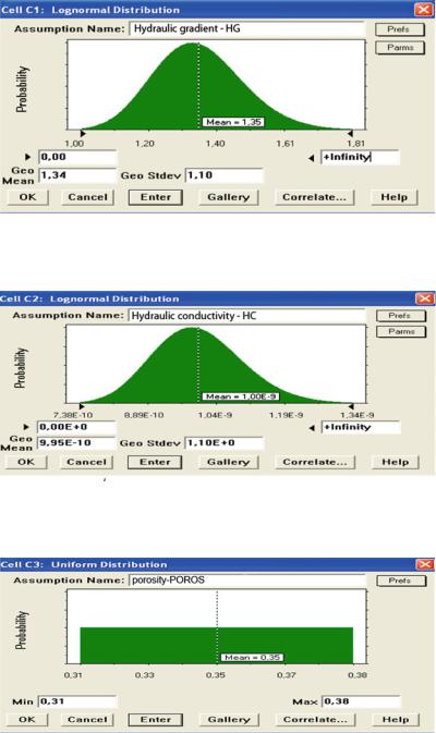
CB software is used to run the simulation. The Distribution Gallery feature (Evans and Olson 1998) allows the user to make the correct choice of probability distribution, in a given research situation. The log-normal distribution curve, being an asymmetrical distribution (positive asymmetry), of the analysed variable, is described by two parameters: the geometric mean mg and the geometric standard deviation sg. In the subsequent chapters of this monograph, the following terminology is used: in the case of log-normal distribution Ð geometric mean mg and geometric standard deviation sg; and as far as the normal distribution is concerned Ð mean value m (instead of: the scale parameter, the expected value of the random variable X, the mean population value), and standard deviation s (instead of: the population standard deviation, shape parameter). Log-normal probability distributions (Figs. 2.3, 2.4, and 2.7) are chosen for approximation of hydraulic gradient (HG), hydraulic conductivity (HC), and diffusion coefÞcient (EDC), whereas random porosity values (POROS) and the thickness of the isolation barrier (TH) are described using uniform distributions (Figs. 2.5, 2.6). Mean values m are consistent with the deterministic values of the variables HC, HD, EDC, TH, and POROS (Table 2.1). The decision to choose log-normal distribution, described using the density function with a range of zero to inÞnity, is based on the work of Schenker et al. (2009), Sonnemann et al. (2004), Rabl and Spadaro (1999), as well as Spadaro and Rabl (2008), and the bibliographies included in the abovementioned publications. Crystal Ball automatically calculates the remaining parameters of lognormal distribution, and these may include: geometric mean mg, geometric standard deviation sg, and minimum as well as maximum values of uniform distributions. The dialog boxes, namely: Log-normal Distribution and Uniform Distribution, and their parameters, which are used in this project, are presented in Figs. 2.3, 2.4, 2.5, 2.6, and 2.7. As can be noticed, the mean value m is higher than the geometric mean value mg of log-normal distribution, a fact thoroughly analysed by Spadaro and Rabl (2008).