systems there is very often no complete information available, or there is no information available regarding the subject of the decision making process. There are different ways of specifying incomplete information and of making decisions under uncertainty. Different management models are used in order to solve the problem of the decision making process, among which the most important ones are (Bubnicki 1993):

•Relational models,2

•Probabilistic models,3

•Game theory models,4

•Fuzzy models.5

As a supplement to the discussion on uncertainty, it may be worth quoting the definition of uncertainty provided in the Regulation of the Minister of Environment of 12 September 2008 (D.U. 2008): “uncertainty can be understood as a parameter, connected with the result of quantity assessment, characterising the diffusion of values, which can be rationally attributed to a given quantity, while considering the impact of both systematic and random factors, and is expressed in percentages of the confidence interval of a mean value equal to 95%, with the inclusion of all asymmetries in the distribution of values”.

4.5Types of Random Variables in Uncertainty Analysis in LCA Studies

By reviewing international subject literature (Frischknecht and Rebitzer 2005; Rabl and Spadaro 1999; Spadaro and Rabl 2008; Hofstetter 1998) and Polish domestic subject literature (D.U. 2008), one could conclude that it is assumed that in the analysis of environmental risk as well as of environmental management, and especially in ecological life cycle assessment, normal distribution and logarithmic-normal distribution, or logarithm-normal, or simply log-normal distribution (Biegus 1999), is used as a characteristic of random variables. The term – log-normal distribution – was first used by Gaddum in 1945 (Statistica 2010; Gaddum 1945; Hofstetter 1998). Since a considerable research potential, dealing with engineering and environmental management, is directed towards analysing

2The relational model specifies the dependence of the decision on its results with the help of certain dependencies, known as relational.

3The probabilistic model uses probability distributions and information regarding the model’s stochastic nature.

4The game theory model (or the “gaming model” – according to Bubnicki) treats the decisionmaker and their parameters as members of a certain game, using the theory of games.

5The fuzzy model formalises inaccurate and fuzzy information.

data, approximated using log-normal distribution, the decision was made to include this distribution in the mainstream of this thesis.

Weidema (1999) draws attention to the fact that random variables that exist in stochastic analyses and studies in environmental protection and economics are usually subject to normal, log-normal, bi-normal, triangular, and uniform distributions. The computer program, offered in the ecoinvent database package (Overview 2007), includes four types of probability distributions: normal, lognormal, triangular, and uniform, while random variables are characterised with the following parameters: mean population value m, standard deviation s (with the 95% confidence level), and diffusion, defined by the range of 2.5–97.5 percentile (Iwasiewicz and Paszek 2004).

In the subject literature, it is possible to come across different approaches to the problem of selecting the probability distribution (function) of variables. For some variables, it is possible to empirically determine probability distributions, whereas for others, such an evaluation is not possible due to the lack of data. It is suggested that probability distributions should be attributed arbitrarily but this solution is met with criticism (Finley et al. 1994; Haimes et al. 1994). At times, it is possible to let the experts decide which probability distribution curve they approve of, yet still, such a decision is a subjective one and provokes controversy (Valopi 1995). A possible solution to the above-mentioned problem may be the employment of the principle of maximum entropy (Jaynes 1957), which has its roots in Laplace’s principle of insufficient reason. It is about defining the probability distribution on the basis of Shannon-Weaver entropy, thanks to which, on the basis of acquired knowledge, one can define the possible shape of the probability distribution curve. This approach does not define the assumptions about the shape of the probability distribution curve, but it chooses the optimal input probability distributions on the basis of limited information in relation to random variables (Tilwari and Hobbie 1976; Lee and Wright 1994). Pio´recki (1973) proposes log-normal distribution as a solution to the problems connected with working time for it approximates the random variable better (working time being the random variable) than normal distribution, because of the reasons mentioned above.

Log-normal distribution is closely connected to normal distribution (Zdanowicz 2002), and it often offers a better approximation of feature distribution than normal distribution, in which the ratios between the values are more important than the differences between them (Morgan and Henrion 1990). The random variable X of the continuous type has a log-normal distribution with parameters m and s with density function (for 0 < x < 1, m > 0, s > 0) when its density takes the form of (see Snopkowski 2007; Zdanowicz 2002; Hoła and Mrozowicz 2003):

where:

m – the mean value

s – standard deviation.

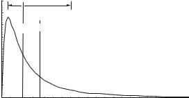
Fig. 4.2 An example of a density function of a log-normal distribution (mg ¼ 1, sg ¼ 3, m ¼ 1.83). The arrows point to a 68% confidence level, geometric mean is denoted as mg, geometric deviation is denoted as sg, and population mean as m (Source: Spadaro and Rabl 2008)

The work of Rabl and Spadaro are of great importance here (Rabl and Spadaro 1999; Spadaro and Rabl 2008), as they thoroughly analyse log-normal distributions. An example of a density function of a log-normal distribution (mg ¼ 1, sg ¼ 3, m ¼ 1.83) can be found in the work of the above-mentioned authors (Fig. 4.2). The arrows point to a 68% confidence level. The geometric mean mg is equal to the median.

As has already been mentioned, log-normal distribution can be very useful in ecological research (risk analysis) or humanities studies, among others (Spadaro and Rabl 2008). It is believed that log-normal distribution is stable, in relation to multiplication (division) of random variables, which means that the distribution of products (quotients) of random variables remains log-normal but with different parameters (Spadaro and Rabl 2008). Log-normal distribution is called by the name of “model of products”, in which the product of random variables X, after finding the logarithm, on the basis of the central limit theorem, provides an expression, in which the sum of these variables will approximately have a normal distribution (logarithms of these variables are random variables as well), and ultimately, the random variable X, whose natural logarithm is subject to normal distribution, has a log-normal distribution (Snopkowski 2007; Benjamin and Cornell 1970). The central limit theorem deserves attention, since it states the measurement of the distribution of an average from a sample for normal distribution independently of population distribution from which the sample was taken (Aczel 2000). Log-normal distribution can also be useful in economic research where variables with positive values are located asymmetrically, in such a way that the values lower than the mode are more clustered while the values higher than the mode are more scattered (Snopkowski 2007). The knowledge of geometric mean, mg, and geometric standard deviation, sg, of probability distributions of input data, may prove useful during the process of defining the confidence intervals. Effective formulas for the multiplicative confidence intervals are provided in the work of other researchers (Sonnemann

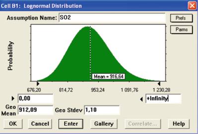
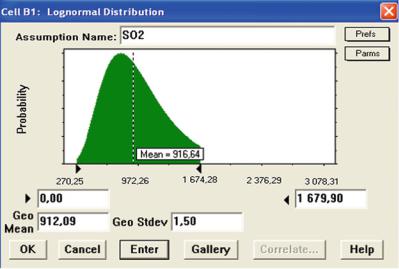
Fig. 4.3 Parameters of log-normal distribution approximating SO2 emissions (Source: Own work)

et al. 2004; Rabl and Spadaro 1999; Spadaro and Rabl 2008; Rabl et al. 2005), and they take the following forms:

where:

mg – mean geometric value

sg – standard geometric deviation.

This approach is illustrated below, based on the example of the emission of SO2, generated during energy production in MSP Power Plant. The data was obtained in 2005. By approximating the SO2 emissions with log-normal distribution, with a range of zero to infinity and its parameters set to the levels shown in Fig. 4.3, where the mean value corresponds to an annual deterministic SO2 emission level amounting to 916.64 Mg, CB software automatically selects the remaining parameters (geometric standard deviation, sg ¼ 1.1, and geometric mean values, mg ¼ 912.09 Mg), which can be entered in the Lognormal Distribution edit window. The results of the MC simulation, with a 10,000-trial randomisation cycle, are shown in Figs. 4.4 and 4.5, respectively, and in the form of statistical reports in Figs. 4.6 and 4.7.

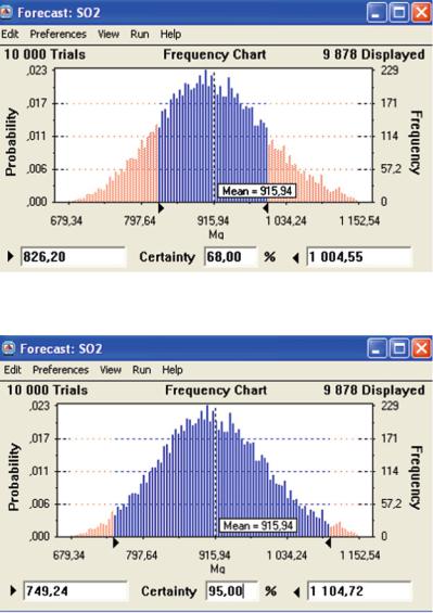
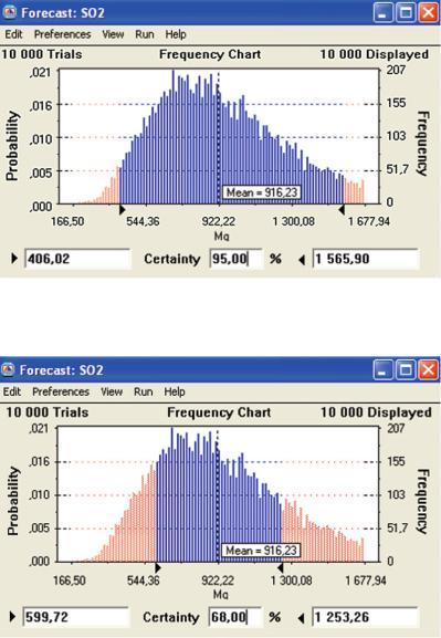
Fig. 4.4 Frequency chart of the SO2 emissions forecast, with 68% confidence interval (Source: Own work)

Fig. 4.5 Frequency chart of the SO2 emissions forecast, with 95% confidence interval (Source: Own work)

The intervals corresponding to the 68% and the 95% confidence level are equal to, respectively:

½826:20; 1004:55& and ½749:24; 1004:72& Mg:

The intervals corresponding to the 68% and 95% confidence level, calculated with the help of formulas (4.1) and (4.2), are equal to, respectively:

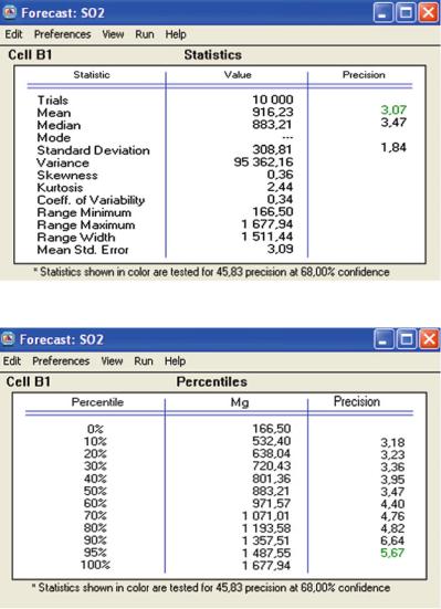
Fig. 4.6 SO2 emissions report – Statistics (Source: Own work)

Fig. 4.7 SO2 emissions report – Percentiles (Source: Own work)

½829:17; 1003:30& and ½753:80; 1103:63& Mg:

It is worth mentioning that, after analysing the results, it can be noted that seven out of eight values describing the span of the confidence intervals, calculated by employing MC simulation with the use of CB package, are smaller than the same values calculated analytically with the help of formulas (4.1) and (4.2). According to Sonneman et al. (2004), dynamic characteristics of a stochastic model can be an explanation of these differences.

Fig. 4.8 Frequency chart of the SO2 emissions forecast, with 95% confidence interval (Source: Own work)

Fig. 4.9 Frequency chart of the SO2 emissions forecast, with 95% confidence interval (Source: Own work)

Simulation results, with geometric standard deviation, sg ¼ 1.5, suggested in literature, for the emission of SO2, are presented in Figs. 4.8 and 4.9 (Sonneman et al. 2004; Rabl and Spadaro 1999). The parameters of the distribution are shown in Fig. 4.10.

Fig. 4.10 Parameters of log-normal distribution approximating SO2 emissions (Source: Own work)

The intervals corresponding to the 68% and the 95% confidence level (Figs. 4.8 and 4.9) are equal to, respectively:

½599:72; 1253:26& and ½406:02; 1565:90& Mg:

The intervals corresponding to the 68% and 95% confidence level, calculated with the help of formulas (4.2) and (4.3), are equal to, respectively:

½608:06; 1368:135& and ½405:37; 2052:203&

The influence of dynamic characteristics of a stochastic model can be noticed here as well.

Log-normal distribution has been used in numerous studies and reports, written by Hofstetter (1998), describing the environmental risk analysis and drawing one’s attention to the fact that this distribution is better at characterising changeability and uncertainty in fate assessment than normal distribution for it cannot take negative values, and so, it can be widely used in LCI analyses, as part of the LCA methodology (e.g. measurements of emissions are never negative – see Hoła and Mrozowicz 2003; Pio´recki 1971; Sonnemann et al. 2004). In order for the significance of this problem to be properly illustrated, the research results concerning the contamination with hazardous waste of the area of a former U.S. Army military base in Ford Ord, California, produced by Valopi (1995), are presented in this monograph. Normal distribution of random variables, such as heavy metals, and especially lead, was used in the simulation. It became clear that, from a statistical point of

view, the result of the simulation (variance), regarding the concentration of lead, was correct, but from an ecological point of view it was unacceptable. The area of the local fauna was much smaller than the research area hence the results were unrepresentative (e.g. negative values were obtained regarding the concentration of the above-mentioned lead). Consequently, the MC simulation results (sensitivity analysis, frequency charts of hazardous substances, etc.), based on the assumptions made and included in the work of Burmaster and Anderson (1994) were questioned and rejected. The decision to use normal distribution was proven incorrect.

Sonneman et al. (2004), in their examination of uncertainty in LCA research, such as the one in the processes of thermal waste utilisation in Tarragona, Spain, in the analysis of input and output sets and in the assessment of the life cycle impacts (impact assessment), make use of normal and log-normal distribution. Tarantola et al. (2008) draw attention to the fact that in the case of domestic data concerning the emissions of industrial gases, approximated with normal distribution, due to the lack of information regarding standard deviation s ¼ 0.1 of the mean value m can be assumed in statistical calculations. In the work of the Society of Environmental Toxicology and Chemistry, SETAC, one can encounter examples of risk assessment in environmental management under uncertainty, for which normal and lognormal distributions are used. Normal and log-normal distributions are used in the description of other processes. Zdanowicz (2002) investigates probability distributions applied in modelling in the Taylor’s program, used, for instance, in simulation modelling of flexible manufacturing cells, and provides examples of application of log-normal distribution in the examination of up time of objects whose defects are caused by gradually increasing fatigue cracks, and used as random models of grain sizes included and seen in a fracture of a metal sample. Log-normal distribution is among these distributions. Biegus (1999) employs normal and log-normal distribution in the probabilistic analysis of load bearing capacity and safety of steel constructions. Layton and Breamer (2009) demonstrate a probabilistic model of transport of contaminants in subsoil using log-normal probability distribution to assess the concentration of microelements (such as lead or arsenic). Crow and Shimizu (1988) analyse and compare computer simulations, which make use of random variables with log-normal, Weibull, and gamma distributions. Tomazi (2004) analyses the problem of deterministic and stochastic optimisation of the production of peptides, used in processes such as the production of synthetic human insulin. In modelling of the kinetic processes of producing peptides under uncertainty, normal and log-normal distributions are employed for the analysed parameters (these are random numbers). The same distributions are chosen for approximation of parameters in modelling of DDT concentration in the environment, using the CliMoChem model for each of the 47 input parameters of the model (Schenker et al. 2009). As mentioned above, log-normal distribution is called by the name of “model of products”. It is calculated on the basis that the random variable, whose natural logarithm is subject to natural distribution, has lognormal distribution (Morgan and Henrion 1990; Snopkowski 2007; Schenker et al. 2009).

In a log-normal distribution, with a positive asymmetry, there are three characteristic values of the random variable X: the modal value (dominant) M0(X), the median x0,5, and the expected value E(X), all of which satisfy the inequality (Tumidajski and Saramak 2009; Hoła and Mrozowicz 2003):

The log-normal curve of the distribution, being an asymmetrical distribution (positive asymmetry) of the analysed variable, is defined using two parameters: geometric mean mg and geometric standard deviation sg. In the subsequent sections of this thesis, in the case of log-normal distribution, the following definitions are used: mg – geometric mean and sg – geometric standard deviation; and in the case of normal distribution: m – mean value (instead of the expected value, the mean population value) and s – standard deviation. Parameters of log-normal distributions are very useful in uncertainty analyses, as they correspond with mean value m and standard deviation s of the normal distribution that describes many processes, despite the fact that the field of density functions of probability distribution is the interval of minus to plus infinity (Snopkowski 2007). Historically speaking, one of the first studies dealing with log-normal distributions were presented by Kołmogorow (1941) and Epstein (1947) who worked on theoretical approach to defining the distributions of grain sizes of product size reductions.

Different definitions of simulation can be found in the subject literature. Łukaszewicz (1975), quoted above, states that “simulation represents the behaviour of the original, through the behaviour of the model”. Naylor (1975), on the other hand, defines simulation as “a numerical technique employed in experiments carried out on mathematical models that illustrate, with the help of a computer, the behaviour of a complex system in a long time interval”. According to Zdanowicz (2002), simulation is a technique used to conduct experiments on certain types of models; it can also be understood as a form of model manipulation, leading to the recognition of the behaviour of the system. Snopkowski (2007) discusses the evolution of the definition of simulation in the last several tens of years. And so, simulations are used especially when solving a problem in an analytical way may be too difficult a process.

As far as normal distributions are concerned, work published by Meier (1997) and the databases developed by the Swiss Federal Institute of Technology in Zurich (ETH), built for Europe, offer normal distributions for the analyses of phenomena occurring in the processes of energy production, such as gas emissions or products or media used in these processes, having the following values of coefficients of variation (CV), serving as relative measures of dispersion (covering the dispersion proportionate to the mean):

•For the data obtained using stochastic methods, CV ¼ 2%

•For, e.g. emission, CV ¼ 10%

•For the remaining data, CV ¼ 20% or 30%.