

70 |
4 Stochastic Analysis of the Environmental Impact of Energy Production |
4.8Description of the Functional Unit of the Boundary System of the Performed Analysis: Inventory Analysis
Functional unit is defined as a quantitative effect of a manufacture system applied as a reference unit in life cycle research. The application of a functional unit ought to be clearly defined and measurable (Kowalski et al. 2007; ISO 14041, 2002). A single product, a group of products, a manufacturing process, or a whole system can be used as a functional unit (Kulczycka and Henclik 2009). The functional unit chosen here is the Power Plant, being a production facility working in an annual cycle. Within the boundaries of the analysed system, the life cycle of the Power Plant presented from the point of view of an annual cycle based on the year 2005 is included. The compiled material-energy balance, shown in Table 4.1, is the basis of the analysis.
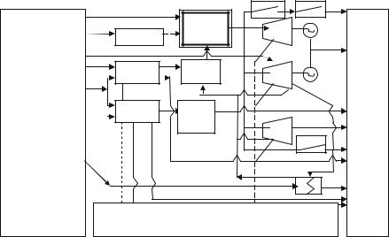
The system boundary is set to establish the source of the materials and the energy that are employed in different individual stages of the process. A precise definition of the system boundary very much depends on the access to data. This knowledge is one of the elements of uncertainty in LCA research. In the case analysed in this section of the thesis, the system boundary is presented in Fig. 4.11.
For the purposes of this analysis some types of waste have been grouped – e.g. worn out devices, elements removed from worn out devices, and insulating materials (not including hazardous substances) have all been categorised as other waste.
In order to define the Power Plant’s environmental impact, the LCA technique has been employed. The LCA issues are currently addressed by more than 40 versions of commercial computer programs. The development of the forecasting model using the LCA technique is supported by SimaPro 7.1 software, developed by a Dutch company – PRe´ Consultants (Goedkoop et al. 2000), and by databases implemented in the software – mostly Ecoinvent. It is one of the best computer software programs on the market that deals with examinations using the LCA technique in terms of its application possibilities and its price (Adamczyk 2004). The program makes use of the concept of components in modelling the life cycle of a product. A component may describe a single part or an entire product comprised of a few components. Eco-indicator 99 has been chosen as an analysis method and, for the purposes of the analysis, own processes have been built as well. The positions 18–43 (inventory table), of the so-called exit, have been defined as Siłownia-E (E-Power-Plant). The remaining entries (positions 44–49) have been described using other processes. For the purposes of the analysis, some types of waste have been grouped – e.g. worn out devices, elements removed from worn out devices, and insulating materials (not including hazardous substances) have all been categorised as other waste.
The analysis does not include methane – emitted to the atmosphere in large quantities during the energy generation processes at the Power Plant complex. Methane is a greenhouse gas mentioned in the emissions trading act; nevertheless, in the analysed period (i.e. the year 2005), methane was not subject to European

4.8 Description of the Functional Unit of the Boundary System of the Performed Analysis 71
Table 4.1 Inventory table for the energy generation processes in the Power Plant Department at the MSP S.A. in 2005
No. |
Minerals and emissions (input and output) |
Quantity |
|
|
|
1. |
Hard coal |
315,680 Mg |
2. |
Blast furnace gas |
4.16 mln GJ |
3. |
Coke oven gas |
0.80 mln GJ |
4. |
Natural gas |
0.08 mln GJ |
5. |
Electric energy |
133,628 MWh |
6. |
Demineralised water |
12,384,404 m3 |
7. |
Tap water |
30,205 m3 |
8. |
Gear oil |
0.80 Mg |
9. |
Solid oil |
0.18 Mg |
10. |
Kotamina |
8.75 Mg |
11. |
Sodium phosphate |
12.4 Mg |
12. |
Hydrated lime |
284.2 Mg |
13. |
Sulphur |
100 Mg |
14. |
Hydrochloric acid |
215 Mg |
15. |
Sodium hydroxide |
219 Mg |
16. |
Conveyor belts |
500 m |
17. |
Land use |
93,055 m2 |
18. |
Carbon dioxide |
1,802.902 Mg |
19. |
Sulfur dioxide |
3,138.1 Mg |
20. |
Nitrogen dioxide |
2,648.5 Mg |
21. |
Dust |
622.1 Mg |
22. |
Chromium |
10.4 kg |
23. |
Cadmium |
1.0 kg |
24. |
Copper |
21.3 kg |
25. |
Lead |
22.8 kg |
26. |
Nickel |
19.6 kg |
27. |
Manganese |
274.0 kg |
28. |
Carbon monoxide |
48.1 Mg |
29. |
Hydrogen chloride |
117.2 Mg |
30. |
Fluorine |
9.36 Mg |
31. |
Aliphatic hydrocarbons |
67.5 Mg |
32. |
Water from cooling cycles |
3,316,958 m3 |
33. |
Municipal sewage |
30,205 m3 |
34. |
Water decarbonisation sediments |
2,289.5 Mg |
35. |
Solutions and sludge from the regeneration of ion-exchange units |
1,528.7 Mg |
36. |
Other sludge and preventive sediments |
10.0 Mg |
37. |
Other engine, gear, and lubricating oils |
15.24 Mg |
38. |
Mineral oils and liquids used as electric insulators and heat carriers not containing |
2.98 Mg |
|
chloro-organic compounds |
|
39. |
Worn out devices containing hazardous substances |
0.132 Mg |
40. |
Lead-acid accumulators and batteries |
2.18 Mg |
41. |
Copper, bronze, brass |
9.842 Mg |
42. |
Aluminium |
0.199 Mg |
43. |
Cables containing crude oil, tar, and other hazardous substances |
11.768 Mg |
44. |
Worn out devices |
3.25 Mg |
45. |
Elements removed from worn out devices |
0.003 Mg |
46. |
Insulating materials |
19.5 Mg |
47. |
Coal fly-ash |
11,272.0 Mg |
48. |
Slag-ash mixtures from liquid drainage of furnace waste |
53,078.1 Mg |
49. |
Unsegregated (mixed) solid municipal waste |
102.0 Mg |
|
|
|
72 |
4 Stochastic Analysis of the Environmental Impact of Energy Production |
ENERGY & MATERIAL RESOURCES
Coke-oven gas
Blast furnace gas
Coal
Crude oil
Water
HCl
NaOH
Calcium hydroxide
Fe2SO4
|
|
RS1 |
RS2 |
PRODU |
|
Steam |
|
|
|
|
TG |
|
CTS |
|
CD |
boilers |
|
||
|
|
|||
|
|
|
||
WDS |
DWS |
TG |
|
Steam |
|
|
|
|
|
|
|
|
|
Electrici |
|
|
|
|
(site) |
WSS |
EHDS |
|
|
|
|
|
TB |
|
Waters |
|
|
|
Pressure |
|
|
|
|
RS3 |
|
|
|
|
Air |
|
|
|
|
|
|
|
|
|
HPB |
|
WASTE (ash, slags), WATER RELEASES, AIR |
EMISSIONS |
Fig. 4.11 A simplified production diagram of the Power Plant department – an element of the boundary system of the energy generation life cycle. CD Coal Deposit (yard) – input: coal, output, conveyor belt, WDS Water Demineralizing Station – input: water, HCl, NaOH, output: demineralizing water, DWS Degassing of the Water Supply – input: condensation water from turbogenerators, WSS Water Softening Station – input: water, output: softening waterm, EHDS Evaporator & Heat network Degassing Station installation – input: degassing water, output: degassing softening water, TG Turbogenerator – input: turbine oil, output U=6 KV, RS1 Reducing Station nr 1 – output: steam 3 MPa, RS2 Reducing Station nr 2 – output: steam 1.6 MPa, RS3 Reducing Station nr 3 – output: 0.8 MPa, TB Turbo blower – output: blow to blast furnace, HPB Heat Power Blanks – output: Steel Plant & Krakow city heating, Steam boilers input: coal from CD, blast furnace gas, coke oven gas, output: steam 9 MPa
trade regulations. If the European Commission recognises the need to limit methane’s emissions, it will then publish the allocation of emissions and the percentage of reduction in the next stage of trade. In addition, methane is not limited in the scope of the allowed emissions levels from individual emission sources and facilities hence it is not included in the application for an integrated permit. It is only subject to charges for the economic use of the environment – for the emissions to the atmosphere. According to the information received from the Department of Environmental Protection at MSP Poland S.A., the amount of methane emitted by the Power Plant complex in 2005 was measured to be 575.08 Mg.
In this analysis it has been taken into consideration that approximately 95% of sewage is recycled and returned to the process.
The amount of energy consumed by the Power Plant is not included in the analysis, as it uses the energy that the Plant itself generates; if that energy were included in the analysis, it would lead to doubling the calculations of the environmental impact of the electric energy generation, since the entire life cycle of the materials and energy sources included in the analysis is taken into account here.
4.9 The Life Cycle Impact Assessment LCA |
73 |
The Life Cycle Inventory analysis (LCI) of the input output set is believed to be one of the most important phases in the LCA method, because in this phase the aim, the scope, the functional unit, the system boundary, and the assumptions are all defined (Roy et al. 2009). The functional unit here applies to the entire manufacture system and the process of production. Defining the system and its boundaries makes it possible to establish the flux of input energy and the materials needed in particular phases of the process.
A simplified production diagram of the Power Plant department is presented in Fig. 4.11.
4.9The Life Cycle Impact Assessment LCA
SimaPro software and the databases (mostly Ecoinvent) implemented in the program have been used in the LCA analysis. Eco-indicator 99 (version H/A) has been the chosen method for the analysis. This method is based on assigning significance to each of the impact categories, which include: carcinogenic agents, climate change, radiation, ozone layer depletion, ecotoxicity, acidification, or eutrophication. Every impact category is assigned with a relevant damage category:
•Consumption of Resources – R,
•Ecosystem Quality – EQ,
•Human Health – HH.
The Eco-indicator method is based on the assumptions similar to the philosophy of G. Taguchi. Here, the losses are replaced by environmental damage caused by the influence of a process or production (Adamczyk 2004). According to G. Taguchi, each quality symbol or parameter may in the case of the process, reach a level where it fulfils the consumer’s expectations to the best of its ability, or, in other words, reaches the optimum quality level. This assumption is also true when it comes to ecological features of a product or environmental parameters. Taguchi uses the so-called loss function, which measures the deviation from its optimum state (Adamczyk 2004; Taguchi and Clausing 1990; Taguchi 1999). In accordance with international standards ISO, every examination employing the LCA technique must include at least the characterisation phase – a phase that is compulsory in the LCA method (Guinee et al. 2001).
The optional elements include: normalisation (calculation of the value of a category indicator in relation to reference information), grouping, measurement, and data quality analysis. These are described in detail in the standard PN-EN ISO 14042 (Environmental Management – Life Cycle Assessment – Life Cycle Impact Assessment – see PN-EN ISO 14042 2002).
74 |
4 Stochastic Analysis of the Environmental Impact of Energy Production |
The outcomes are presented in the form of results in the following phases:
•Characterisation – it relies on the calculation of the value of a category indicator for the LCI results and makes it possible to evaluate the influence level of the method in a quantity dealing with the given impact category. The characterisation parameter in the Eco-indicator 99 method is defined on the basis of the so-called intermediate points. This method relates the impact of harmful activity on natural environment to three damage categories: Human Health, Ecosystem Quality, and Consumption of Resources (Simapro 2007). Damage to human health is expressed in DALY units – they describe Disability Adjusted Life Years. Murray and Lopez introduced DALY units in 1996 for the World Bank and World Health Organisation (WHO). They allow us to determine the relative amount of time by which human life is shortened as a result of damaging waste management effects. The analysis of harmfulness involves making a connection between the health impact and the final value of the DALY indicator, considering the number of years lost due to disability (YLD) and the number of years of life lost (YLL) (Adamczyk 2004).
The damage to the quality of the ecosystem (eco-toxicity) is expressed as a percentage of species disappearing from a given area, as a result of the influences on the environment. The reference unit used here is the Potentially Affected Fraction (PAF), expressed as a percentage. If there is a need to express acidification and eutrophication, the Potentially Disappeared Fraction units are used (PDF). The unit that expresses the damage done to the ecosystem is PDF, related to the area of the ground in a year: PDF*m2*year (Adamczyk 2004). The reduction of natural resources is assessed by analysing the quality of the natural sources that have not yet been extracted, including fossil fuels. The surplus energy (MJ) is necessary to access the useful minerals, which may be extracted at a lower cost. An in-depth description of the Eco-indicator 99 method can be found in the work of: Kowalski et al. (2007) and SimaPro (2007).
•Normalisation – it relies on the division of the value of the impact category by the impact on the environment per 1 European inhabitant in a year, i.e. nondesignated values. Normalisation facilitates interpretation and understanding of measurement.
•Weighting – the result of normalisation is multiplied by the appropriate subjective significance coefficient – significant values are expressed in eco-points [Pt] and in submultiples [mPt] – mili-points.
Eco-point is a unit that informs us of the effects that one (on average) European inhabitant has on the environment in 1 year. It is calculated by dividing all of the European emissions by the number of its inhabitants. It is worth mentioning the fact that the value of an eco-point [Pt] should be a dimensionless number and that it is created by dividing the entire environmental load, shared by the European continent, by the number of its inhabitants, and multiplying the obtained answer by 103 (Goedkoop et al. 2000).
4.10 Stochastic Analysis of the Environmental Impact of the Four Scenarios |
75 |
By presenting the outcomes of the analysis one may wish to relate them to the three damage categories:
•Human Health, part of which are factors, such as the number and duration of diseases, premature deaths caused by the environmental impact, as well as effects such as climate change, ozone layer depletion, carcinogenic agents, influence of radiation, or difficulties with respiratory processes.
•Ecosystem Quality, which includes the influence on the variety of species, especially vascular or smaller plants, and on the following effects: eco-toxicity, acidification, eutrophication, and land use.
•Consumption of Resources, which includes the surplus energy needed in the past to extract minerals and fossil resources of worse quality; on the other hand, the impoverishment of building minerals, such as gravel or sand, is treated as land exploitation (Adamczyk 2004).
or to 11 impact categories which add up to the relevant damage categories, i.e. carcinogenic agents, the effects on respiratory systems of organic compounds, the effects on respiratory systems of non-organic compounds, climate change, radiation, ozone layer depletion (Human Health), eco-toxicity, acidification/eutrophication, land use (Ecosystem Quality), mineral and fossil fuel consumption (Consumption of Resources).
The process of defining the eco-point [Pt] is carried out in three steps, according to the diagram proposed by Adamczyk (2004). In inventory analysis new processes are established or existing processes, included in SimaPro 7.1 library, are used. Complete results of the performed LCI analysis (presented here – Ocena 2008), take the form of the following types of frequency charts: characterisation (in a division into 11 impact categories), normalisation (in a division into 3 damage categories), and measurement (in a division into 11 impact categories).
4.10Stochastic Analysis of the Environmental Impact
of the Four Scenarios of Energy Generation Processes in MSP Power Plant
The results of the LCA analysis have been used here to present the stochastic analysis of the environmental impact of the four scenarios of energy generation processes in MSP Power Plant. In order to assess the credibility of the LCA results, which are burdened with a certain degree of uncertainty, the probabilistic analysis, based on the combination of MC simulation as well as sensitivity and uncertainty analysis, has been used with the aim of evaluating the uncertainty in LCA. This thesis is of methodical nature and the simulation results presented here are of cognitive and applied importance. Therefore, it is worth supporting this work with complete results of the LCA analysis (in which the author took part in the inventory phase), which form the basis for the subject analysis, demonstrated in this work.
76 |
4 Stochastic Analysis of the Environmental Impact of Energy Production |
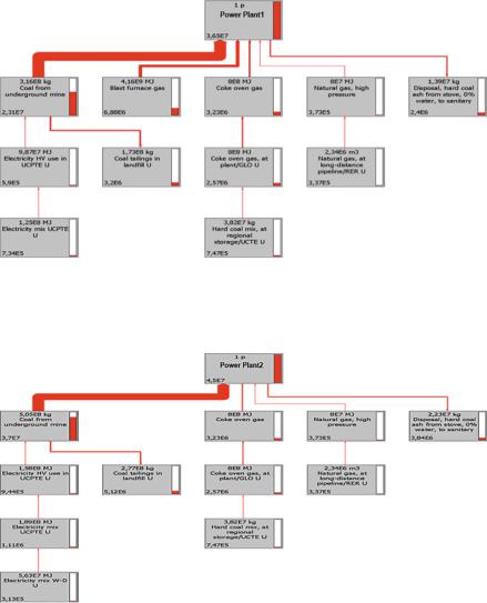
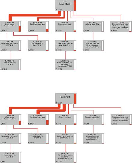
A fundamental element of the LCI life cycle phase in SimaPro 7.1 is the creation of the tree of processes, depicting all of the vital life cycle processes and the correlations between them. The tree of resources and processes is presented in the form of boxes; each tree element includes a piece of information regarding the involvement of the processes and materials, proportionate to the value of indicators – it is possible to determine which process/material influences the product the most; it is also possible to define the participation of a single element in the entire life cycle. The structure of the tree allows the user to see a detailed review of the resources and their participation in the processes. Each tree box is equipped with a bar chart (or thermometer), which indicates the participation of resources in relation to the value of indicators (Kulczycka 2001). The thickness of the arrows, as well as the height of the bars, is connected to the size of the environmental impact. The trees may be presented separately for each of the damage categories or together as a single score.
By using the process trees one can examine positive impacts on the environment – these, in SimaPro 7.1, are represented by green bars next to the given elements of the process tree. The red bars, on the other hand, indicate that the impact on the environment is negative (Kulczycka 2001; Goedkoop et al. 2000).
In this analysis, the data presented in Table 4.2, showing measurement results, is employed. The table has been created using the data obtained from SimaPro 7.1 library, which makes use of the coefficients included in the Eco-indicator 99 method, the data from the inventory table for the energy generation processes in the Power Plant department, included in Table 4.1. It also includes processes mentioned above, created for the purposes of the analysis, and originating from the LCA study designed for the purposes of the postdoctoral thesis by the Mineral and Energy Economy Research Institute of the Polish Academy of Sciences in Krako´w (Ocena 2008).
A comparative analysis for the four scenarios of the Power Plant’s annual work cycle has been performed, taking into consideration that the scenarios differ only in the change of proportioning ratios of the two types of fuels: hard coal and blast furnace gas (the remaining fuels, such as natural gas and coke oven gas are left at their current levels – they are used as start-up gas owing to their higher heating value). The simulation has been conducted with an assumption that 1 GJ of energy from coal is equal to 1 GJ of energy from other fuels:
•Scenario S1 – in 2005 – 62% of energy comes from hard coal, 38% from blast furnace gas,
•Scenario S2 – an assumption that 100% of energy comes from hard coal,
•Scenario S3 – an assumption that the percentages of fuels are even,
•Scenario S4 – an assumption that 30% of energy comes from hard coal, 70% from blast furnace gas.
In order for a cumulative impact factor to be determined, a summary of all indicators has been performed, and is included in the TOTAL column. The results of the analysis are expressed using eco-points [Pt], a unit accepted in the LCA method (see Sect. 4.9 for more information) that explicitly defines the measurement of environmental impacts. As is emphasised by Merkisz et al. (2007), the positive

4.10 Stochastic Analysis of the Environmental Impact of the Four Scenarios |
77 |
Table 4.2 The results of the LCA analysis in the four scenarios of the Power Plant’s annual work cycle, divided into 11 impact categories
Impact category |
Unit |
Scenario 1 |
Scenario 2 |
Scenario 3 |
Scenario 4 |
Carcinogenicity |
Pt |
5,436,453.7 |
8,648,551 |
4,367,048.9 |
2,654,440 |
Respiratory system – |
Pt |
14,024.572 |
15,912.46 |
13,396.037 |
12,389.466 |
organic compounds |
|
|
|
|
|
Respiratory system – non- |
Pt |
14,680,447 |
20,792,656 |
12,645,508 |
9,386,634.4 |
organic compounds |
|
|
|
|
|
Climate change |
Pt |
10,448,258 |
7,001,483 |
11,595,807 |
13,433,532 |
Radiation |
Pt |
16,528.649 |
24,134.59 |
13,996.4 |
9,941.1081 |
Ozone layer |
Pt |
499.6735 |
635.9435 |
454.30506 |
381.6494 |
Eco-toxicity |
Pt |
316,502.38 |
485,314.1 |
260,299.82 |
170,293.71 |
Acidification/ |
Pt |
1,514,979.8 |
2,116,324 |
1,314,774.5 |
994,153.29 |
eutrophication |
|
|
|
|
|
Land use |
Pt |
242,279.63 |
336,367.2 |
210,955.03 |
160,789.98 |
Minerals |
Pt |
22,744.293 |
23,468.29 |
22,503.256 |
22,117.237 |
Fossil fuels |
Pt |
3,855,978.8 |
5,544,591 |
3,293,788.3 |
2,393,463.6 |
TOTAL – summary of |
Pt |
36,548,696.5 |
44,989,437 |
33,738,532 |
29,238,136 |
influence |
|
|
|
|
|
TOTAL – summary of |
Pt |
36,510,598.74 |
44,953,891.94 |
33,699,465.59 |
29,200,035.13 |
influence ¼ mg |
Pt |
36,419,105.46 |
44,793,382.60 |
33,607,403.62 |
29,121,534.18 |
x0,5 |
|||||
mg – geometric mean |
|
|
|
|
|
x0,5 – median |
|
|
|
|
|
value of eco-points indicates a negative impact on the environment (the higher the value expressed in [Pt] the greater the negative impact), while the negative values mean environmental benefits.
In the S1 scenario, which describes the present state (and in 2005), where 62% of energy comes from hard coal and 38% from blast furnace gas, the Power Plant’s environmental impact in a 1-year production cycle is potentially high – 36,548,697 Pt.
The S2 scenario is a theoretical scenario, in which the only boiler that is heated with coal is boiler no. 8, produced in Poland (OP-230 Boiler). In this scenario the cumulative impact factor of the Power Plant amounts to 44,989,437 Pt.
In the third scenario (S3) based on an assumption that the fuels are dosed equally, the total influence of the Power Plant amounts to 33,738,532 Pt.
The fourth and final scenario (S4) assumes minimal amount of energy involved that comes from hard coal. This is due to the fact that the majority of the boilers are adapted to burn pulverised coal (or coal dust), and such boilers cannot work under a certain critical amount of dust, as it would lead to boiler shutdown. In this scenario the cumulative impact factor of the Power Plant is 29,238,136 Pt.
This means that the energy generation processes during a 1-year cycle of the Power Plant cause the same amount of pollution as 36,548.7 Europeans (scenario 1), 44,989.4 Europeans (Scenario 2), 33,738.5 Europeans (Scenario 3), and 29,238 Europeans (Scenario 4) cause in a year.
The process trees are presented in Figs. 4.12–4.15 (Ocena 2008). The tree boxes also show the share of each of the processes in the total impact on the environment
78 |
4 Stochastic Analysis of the Environmental Impact of Energy Production |
Fig. 4.12 The developed view of the resources and processes tree for the Power Plant (annual data) – scenario S1 – present state – 62% of energy comes from hard coal, 38% from blast furnace gas. In Figs. 4.12–4.14, the E5, E6, and E7 symbols mean 105, 106 and 107 (Source: Ocena (2008) based on data from MSP)
Fig. 4.13 The developed view of the resources and processes tree for the Power Plant (annual data) – scenario S2 – an assumption that 100% of energy comes from hard coal. There is no box containing blast furnace gas (Source: Ocena (2008) based on data from MSP)
(in the bottom left corner), as well as simultaneously present these data on a bar chart, which can be found in each of the boxes. The total result of such influences is given in the first box.
The allocation of emissions has been made on the basis of data received from both the Department of Environmental Protection at MSP S.A. Power Plant (Wniosek 2006) and the subject literature data (Lorenz 1999).
4.11 Defining Input Data: Organising the Simulation |
79 |
Fig. 4.14 The developed view of the resources and processes tree for the Power Plant (annual data) – scenario S3 – an assumption that fuels are dosed in equal percentages (Source: Ocena (2008) based on data from MSP)
Fig. 4.15 The developed view of the resources and processes tree for the Power Plant (annual data) – scenario S4 – an assumption that 30% of energy comes from hard coal, 70% from blast furnace gas (Source: Ocena (2008) based on data from MSP)
4.11Defining Input Data: Organising the Simulation
Before a simulation can be run it is necessary to define input information received in graphic form. The analysis consists of 11 impact categories (influences) and their total impact on the environment (Table 4.2).
80 |
4 Stochastic Analysis of the Environmental Impact of Energy Production |
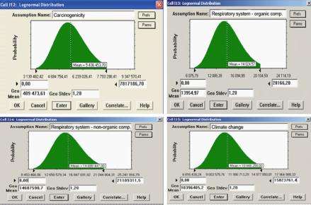
In all of the discussed scenarios (1–4), the simulations have been performed using Crystal Ball software, in accordance with the steps discussed in Chap. 2. In order for the algorithm to be run, it is necessary to be aware of probability distribution, which is applied in stochastic analysis of environmental impact of energy production processes at MSP, thanks to which at least a theoretical reflection of the analysed real process can be performed. In the field of statistical analysis of uncertainty in the problems of ecology, the most important work has bee published by Sonnemann et al. (2004), Rabl and Spadaro (1999), Spadaro and Rabl (2008), and the Eco-indicator 99 method developed by a Dutch company PRe´ Consultants. From the analysis of the above-mentioned projects, it can be concluded that random values of the impact category, in stochastic LCA analysis defining the impact of the energy production processes in the Power Plant on the environment, may be described using log-normal distribution with standard geometric deviation sg ¼ 1.2. The Lognormal Distribution tab windows that contain log-normal distributions of each of the eleven impact categories of the analysed scenarios, are presented in Figs. 4.16–4.19, respectively. The distribution tabs define the standard geometric deviation sg and the mean value m that correspond to the random values of the impact category (Table 4.2), which are approximated with log-normal distributions. CB program automatically “matches” the distribution, calculating its remaining parameters: geometric mean mg and the upper boundary of log-normal distribution. The lower boundary ¼ 0. As can be observed in Figs. 4.16–4.19, lognormal distributions are cut off on the right-hand side.
Fig. 4.16 (continued)
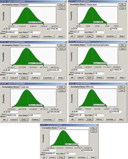
4.11 Defining Input Data: Organising the Simulation |
81 |
Fig. 4.16 The log-normal probability distributions tabs for the 11 impact categories, available in Crystal Ball software for the S1 scenario (Source: Own work)
Scenario S1 – present state – 62% of energy comes from hard coal, 38% from blast furnace gas.
Scenario S2 – an assumption that 100% of energy comes from hard coal. Scenario S3 – an assumption that fuels are dosed in equal percentages. Scenario S4 – an assumption that 30% of energy comes from hard coal, 70%
from blast furnace gas.