

Kluwer - Handbook of Biomedical Image Analysis Vol
.1.pdfA Basic Model for IVUS Image Simulation |
43 |
(a) |
|
(b) |
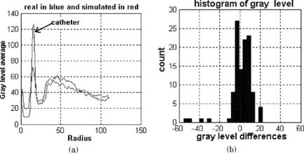
Figure 1.39: Real (blue) and simulated (red) gray-level vertical profile (a) of ROIs of Fig. 1.38(b) and data correlation (b).
The maximal difference profiles are localized in the transducer sheath graylevel distribution and the baseline of the transducer sheath inner region. These differences can be smaller, increasing the video and instrumental noise. The high-frequency oscillations in the gray-level profiles come from the concentric arterial structures. We can also observe the gradual reduction of the gray-level magnitude from intima/media interface to adventitia, caused by the ultrasound intensity attenuation.
(a) |
|
(b) |
|
|
|
Figure 1.40: Global projections in the direction θ (a), from Figs. 1.38(b) and
(d) and the corresponding histogram gray-level differences (b).
44 |
Rosales and Radeva |
Figure 1.41: Global projection in the R direction (c), from Figs. 1.38(b) and (d), the corresponding histogram gray-level differences are shown in (b).
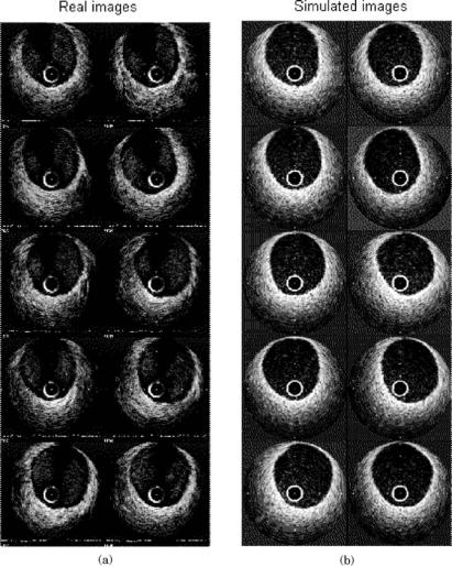
The next step in the validation of the model is to show the significant correspondence between real and simulated gray-level distribution data in the medical zones of interest. For this purpose, 20 validated real IVUS images and their corresponding ROIs were selected. The spatial boundaries of the morphological structures of the real data are kept in the synthetic data. Figure 1.42(a) shows ten real IVUS images and their corresponding simulated (b) synthetic images. The polar images are shown in Fig. 1.43.
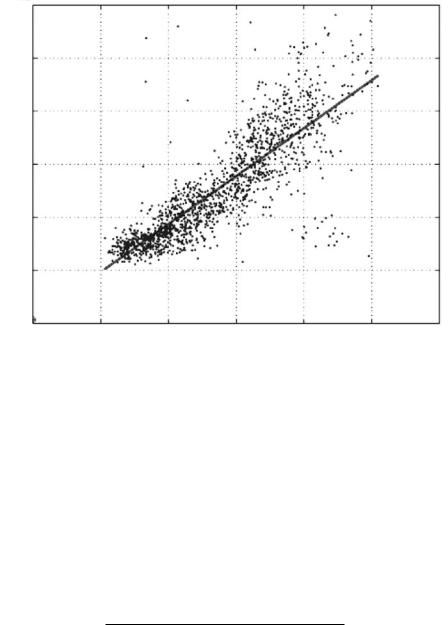
Figure 1.44 shows the simulated versus real gray-level correlation for the polar ROIs images selected as shown in Fig. 1.38. The linear correlation coefficients show a good gray-levels correspondence, these being m = 0.90 and b = 1.42. The best correspondence is located by low gray levels (20–40 gray levels), lumen scatterers, lumen/intima transition, and adventitia. The transitions of intima/media and media/adventitia (45–60 gray levels) indicate gradual dispersion. The CNRS average presents significative uniformity values, µ = 6.89 and σ = 2.88, for all validated frames. The CNRS as figure of merit for each arterial validated region is shown in Fig. 1.45. The CNRS region mean, standard deviation, and the SSE values referring to the 20 image frames are summarized in Table 1.5. The lumen is a good simulated region, with mean µ = 0.46 and deviation σ = 0.42. The explanation is that the lumen is not a transition zone, the attenuation ultrasound intensity in this region is very poor (1–2%), which determines a simple gray-level profile.
A Basic Model for IVUS Image Simulation |
45 |
(a) |
|
(b) |
Figure 1.42: Ten original IVUS images (a) and the corresponding simulated (b) images.
The histograms of gray-level differences for each region of interest in the 20 validated frames are displayed in Figs. 1.46 and 1.47. Table 1.6 explains the distribution center µ and the standard deviation σ for the gray-level difference distribution for each simulated region. The minus sign in the mean values means that the simulated images are brighter than the real images. A symmetric Gaussian can be seen in the lumen gray-level differences distribution, with mean µ = −2.44 and deviation σ = 15.13. The intima distribution has
46 |
Rosales and Radeva |
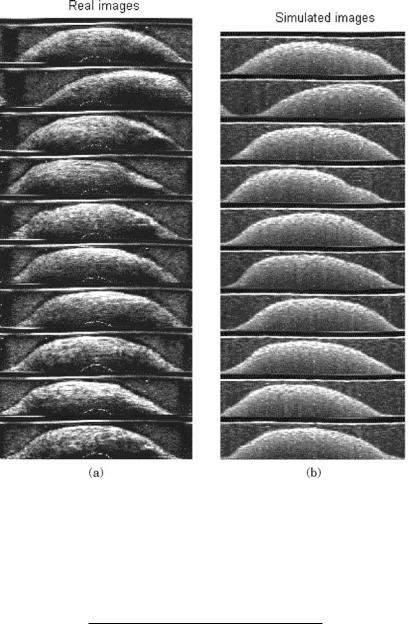
Figure 1.43: Ten polar real images (a) and the corresponding simulated
(b) images.
Table 1.5: CNRS mean, standard deviation (std), and sum square error for different tissues structures
ROI |
Mean |
Std |
SSE |
|
|
|
|
Lumen |
0.46 |
0.42 |
47.68 |
Intima |
10.0 |
4.38 |
12.63 |
Media |
9.91 |
5.14 |
15.05 |
Adventitia |
7.21 |
2.76 |
4.28 |
|
|
|
|
A Basic Model for IVUS Image Simulation |
47 |
Simulated gray level
120
[m, b] = [0.90, 1.42]
100
80
60
40
20
0 |
20 |
40 |
60 |
80 |
100 |
120 |
0 |
real gray level
Figure 1.44: Simulated versus real gray-level values for 20 ROIs comparing pixel gray-level and the regression line.
a mean of µ = −18.56 and deviation of σ = 24.01, and the media region has a mean of µ = −17.82 and a deviation of σ = 22.62. The gray-level differences distribution displays a light asymmetry. As a result, the simulated image tends to be brighter than the real image. The adventitia gray-level differences values show a symmetric distribution with a center of µ = −13.30 and a deviation of
σ = 14.27.
Table 1.6: Mean and deviation of the ROIs gray-level differences referred from histograms in Figs. 1.46 and 1.47
ROI |
µ |
σ |
|
|
|
Blood |
−2.44 |
15.13 |
Intima |
−18.56 |
24.01 |
Media |
−17.82 |
22.62 |
Adventitia |
−13.30 |
14.27 |
48 |
Rosales and Radeva |
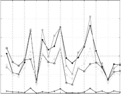
CNRS Vs for each ROI's in the validated frames
25
r(+) (Blood) b(*) (Intima) g(s) Media)
m(c) (Adventitia) 20 y(d) (Average)
15
CNRS
10
5
0
0 |
2 |
4 |
6 |
8 |
10 |
12 |
14 |
16 |
18 |
20 |
|
|
|
|
Validated frames |
|
|
|
|
|
|
Figure 1.45: CNRS values for each ROI of 20 manually segmented image frames.
It is very important to note that the gray-level difference distribution exhibited Gaussian distributions for all regions of interest. Certainly, the synthetic image brightness is an open problem of the image formation model. The simplest approach is to variate it by modifying the original intensity
Io of the ultrasound beam, similar to the offset of the image acquisition system. Real and simulated gray-level distributions for each region of interest are shown in Figs. 1.48 and 1.49. We can note the great similarity in the gray-level distributions profile. Figure 1.50 shows the gray-level histogram of the different tissues structures that appear in IVUS images. As expected, it can be seen that the gray-level distributions of different structures overlap and as a result it is not possible to separate the main regions of interest in IVUS images, using only the gray-level distributions as image descriptors.

A Basic Model for IVUS Image Simulation |
49 |
Figure 1.46: Histogram of gray-level differences for lumen (a) and intima (b).
Figure 1.47: Histogram of gray-level differences for media (a) and adventitia
(b).
(a) |
(b) |
Figure 1.48: Real (blue) and simulated (red) gray-level distributions for lumen
(a) and intima (b).

50 |
Rosales and Radeva |
(a) |
(b) |
Figure 1.49: Real (blue) and simulated (red) gray-level distributions for media
(a) and adventitia (b).
Figure 1.50: Simulated gray-level distributions for blood, intima, media, and
adventitia.
A Basic Model for IVUS Image Simulation |
51 |
1.7 Conclusions
Although IVUS is continuously gaining in use in practice due to its multiple clinical advantages, the technical process of IVUS image generation is not known to doctors and researchers developing IVUS image analysis. This fact leads to a simplified use, analysis, and interpretation of IVUS images based only on the gray-level values of image pixels.
In this chapter we discuss a basic physical model to generate synthetic 2D IVUS images. The model has different utilities: Firstly, an expert can generate simulated IVUS images in order to observe different arterial structures of clinical interest and their gray-level distribution in real images. Secondly, researchers and doctors can use our model to learn and to compare the influence of different physical parameters in the IVUS image formation, such as the ultrasound frequency, the attenuation coefficient, the beam number influence, and the artifact generations. Thirdly, this model can generate a large database of synthetic data under different device and acquisition parameters to be used for validating the robustness of image processing techniques. The IVUS image generation model provides a basic methodology that allows us to observe the most important real image emulation aspects. This initial phase does not compare pixel to pixel values generation, showing the coincidence with the real image, but looks for a global comparison method based on gray-level difference distribution. The input model applies standard parameters that have been extracted from the literature. Hence this model is generic in the sense that the model allows simulation of different processes, parameters, and makes it possible to compare to real data and to justify the generated data from the technical point of view.
The model is based on the interaction of the ultrasound waves with a discrete scatterer distribution of the main arterial structures. The obtained results of the validation of our model illustrate a good approximation to the image formation process. The 2D IVUS images show a good correspondence between the arterial structures that generate the image structures and their gray-level values. The simulations of the regions and tissue transitions of interest lumen, lumen/intima, intima/media, media/adventitia and adventitia, have been achieved to a satisfactory degree. Interested readers are invited to check the generation model in http://www.cvc.uab.es/ misael.
52 |
Rosales and Radeva |
Questions
1.Which qualitative phenomenon and parameters are possible to observe using the IVUS technique?
2.Which principles is IVUS data acquisition based on?
3.What are the principal limitations of the IVUS technique?
4.How is the distance to reflecting object by ultrasound technique determined?
5.What is attenuation coefficient?
6.What are axial and radial resolution?
7.What is the usual IVUS resolution?
8.How many scatterers structures are taken into account by a basic IVUS image model?
9.How are 1D and 2D echograms generated?
10.What are the steps followed in the generation of an IVUS image?