

Kluwer - Handbook of Biomedical Image Analysis Vol
.1.pdf64 |
Wong |
0 |
t1 |
|
|
VT |
|
VA |
Pulse |
|
|
|
generator |
Detector A
|
Gate-pulse |
|
|
generator |
|
|
A |
|
|
Logic unit |
|
|
B |
|
Region of |
Gate-pulse |
|
coincidence |
||
generator |
||
detection |
||
Detector B |
|
|
Pulse overlap |
|
|
=> coincidence |
|
A |
|
|
B |
Coincidence |
|
window = 2τ |
||
|
||
|
t |
|
|
t1t2 |
|
Pulse |
t2 |
generator |
0 |
|
VT |
|
VB |
|
= |
Positron annihilation |

 = Accepted by coincidence detection


 = Rejected by coincidence detection
Figure 2.2: Annihilation coincidence detection. The two gamma-ray detectors are placed at the opposite ends of the object to detect the photons that originate from the positron annihilation site. The event is registered if the annihilation occurs within the region of coincidence detection of the detector pairs. If the gamma rays originate outside the region of coincidence detection of the two detectors but only one of the photons is detected, the event is not registered as the detection of a single photon violates the condition of coincidence.
coincidence detection [21], which is unique to PET imaging. It should be noted, however, that the condition of coincidence (or simultaneity) is not achievable in practice, and a coincidence resolving time (or a coincidence timing window) of less than 15 ns is often used to account for differences in arrival times of the
Quantitative Functional Imaging with Positron Emission Tomography |
65 |
two gamma rays, time taken to produce scintillation light in the detector, and time delays in the electronic devices in the PET system.
Once the signal leaves the detector module, it is processed by several electronic circuits. The choice of components depends upon the application and, therefore, there are many ways to implement the coincidence detection circuitry. A simplified schematic representation of detecting coincidence events with two detectors is also shown in Fig. 2.2. The output signal from each detector is fed into a pulse generator. Note that the signal amplitude from the two detectors (VA and VB) may not be the same due to incomplete deposition of photon energies or variation in efficiency among the detectors. In addition, there exists a time difference between the detectors to react upon the photons arrival, and a finite reaction time for the electronic devices to response, resulting in difference in the time t1 and t2 at which the amplitude of the signal crosses a certain fixed voltage level (VT ), which triggered the pulse generator to produce a narrow pulse. The narrow pulse is then fed into the gate-pulse generator where a pulse of width 2τ (coincidence timing window) is generated for individual detectors. A coincidence detection circuit is then used to check for a logical AND between the incoming pulses. For the example shown in Fig. 2.2, there is a pulse overlap between two signals produced by the gate-pulse generators. Therefore, the event is a true coincidence which is regarded as valid and is registered. It is easy to see that if t2 − t1 ≥ 2τ , the event is not in coincidence, and thus it is not recorded by the coincidence detection circuit.
2.6 Coincidence Criteria
In general, an event (positron annihilation/photon emissions) is regarded as valid and is registered by the coincidence detection circuit if the following criteria are satisfied [26, 53]:
two photons are detected within a predefined coincidence window,
the LoR formed between the two photons is within a valid acceptance angle of the tomograph, and
the energy deposited in the crystal of the detector by both photons is within the selected energy window.
Such coincident events are often referred to as prompt events.
66 |
Wong |
2.7 Detectors
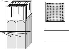
To image the distribution of positron-emitting isotope in the body, both of the 511 keV photons emitted from positron annihilation must be detected in coincidence. Unlike other instruments used in nuclear medicine, PET uses electronic rather than lead collimators to detect signal (event) results from annihilation of the positron and an electron. The probability of detecting both photons depends on the detector efficiency, which is strongly related to the stopping power of the scintillator and the thickness of the scintillator used in the detector. Early generation of PET scanners used NaI(Tl) crystals, the same material used in gamma camera. Modern PET scanners use much denser scintillators, such as bismuth germanate oxide (BGO) [27], which has been the scintillator of choice for more than two decades due to its very high density and stopping power for the 511 keV gamma rays. In order to provide higher detection efficiency and spatial resolution with lower production cost, a number of detector designs were proposed in the 1980s and the most successful one was the block detector technique proposed by Casey and Nutt, using BGO crystal [28]. A typical BGO block detector comprises a rectangular block consisting of between 6 × 8 and 8 × 8 individual scintillation crystals, attached to an array (usually 2 × 2) of photomultiplier tubes (PMTs) at which the scintillation light is amplified and converted into electrical signal for the coincidence detection circuit to register. A schematic outline of such a block detector is shown in Fig. 2.3. The BGO element in which a gamma ray interacts is determined by the relative light output
Scintillator
array
PMTs |
X =
P1 + P2 - P3 - P4
P1 + P2 + P3 + P4
Y =
P1 - P2 + P3 - P4
P1 + P2 + P3 + P4
Figure 2.3: Schematic diagram of a BGO block detector commonly used in
commercial PET systems.
Quantitative Functional Imaging with Positron Emission Tomography |
67 |
from the four PMTs. Anger-logic is used to obtain the X and Y positions based on the four PMT outputs Pi:
X |
= |
P1 |
+ P2 |
− P3 |
− P4 |
(2.4) |
||
P1 + P2 + P3 + P4 |
||||||||
|
|
|||||||
Y |
= |
P1 |
− P2 |
+ P3 |
− P4 |
|
(2.5) |
|
P1 + P2 + P3 + P4 |
||||||||
|
|
|||||||
The combined BGO block/photomultiplier system has an approximately cubic spatial resolution of 4 mm full-width-at-half-maximum and coincidence timing window of approximately 12 ns.
As seen from Fig. 2.2, the probability that the annihilation event occurs exactly within the region of coincidence detection and is recorded by the detectors is very small because most gamma rays may travel out of the region of coincidence detection even if the annihilation event occurs within that region. This probability can be increased by using a ring of detectors within which any detector is in coincidence with all other detectors located at the opposite side of the ring. With the use of multiple rings of detectors, the probability of coincidence detection is further increased because coincidences can be detected by other rings of detectors if they cannot be recorded by the plane of the ring within which the annihilation events occur. The device that used to detect the 511 keV gamma rays emitted from annihilation and construct a map of radiopharmaceutical distribution inside the body is called tomograph (or scanner), which usually has multiple rings of detectors surrounding the patient.
2.8 Detected Events
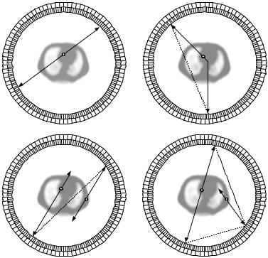
Ideally the only prompt events registered by the detectors are those which arise from “real” positron annihilation. However, a number of other unwanted events that satisfied the coincidence criteria are also registered. The detection of unwanted events causes noise and degradation in spatial resolution. Therefore, their correction is essential to improve the quantification. In general, five types of event can be detected by PET scanner, and four of them are illustrated in Fig. 2.4.
A true coincidence refers to an event that two photons are emitted back- to-back from a single positron–electron annihilation, and are detected simultaneously by opposing detectors within the region of coincidence detection and within the coincidence timing window of the system.
68 |
Wong |
(A) |
(B) |
(C) |
(D) |
Figure 2.4: Types of coincidence event recorded by a full-ring PET system. The white circle indicates the site of positron annihilation, and the solid line represents the gamma ray, (A) true coincidence, (B) scattered coincidence, (C) random (or accidental) coincidence, and (D) multiple coincidence. The mispositioned line of response is indicated by the dashed line.
Scattered coincidence occurs when one or both of the emitted photons undergo a Compton scatter interaction in tissue. Compton scattering causes a loss in energy of the photon and change in direction of the photon. Since the direction is changed, the origin where the photons were emitted cannot be located correctly and, as a result, the event is mispositioned, leading to decreased contrast and deteriorated quantification.
A random (or accidental) coincidence occurs when two unrelated photons, which have not originated from the same site of positron annihilation, strike opposing detectors within the coincidence timing window. Since the random events are produced by photons emitted from unrelated decays, they are spatially uncorrelated with the activity distribution. The random coincidences are
Quantitative Functional Imaging with Positron Emission Tomography |
69 |
a source of noise, the rate of which is approximately proportional to the square of the activity in the field of view (FOV). The performance of PET scanner for high count rate studies is degraded and therefore, correction for randoms is necessary.
Multiple events are similar to random events, except that three photons originated from two positron annihilations are detected within the coincidence timing window. Because of the ambiguity in positioning the event, these coincidences are normally discarded.
A single event for which only one photon is emitted is also possible due to some physical factors. The single events are usually rejected by the coincidence detection circuit since detection of only one event within the timing window violate the condition of coincidence. Yet in practice, about 1–10% of single events are converted into paired coincidence events.
2.9 Data Acquisition
Most of the modern PET tomographs are capable of acquiring data in two different modes: two-dimensional (planar) acquisition with septa in-place and three-dimensional (volumetric) acquisition with septa retracted, exposing the detectors to oblique and transaxial annihilation photon pairs. Both modes of configuration for data acquisition are shown in Fig. 2.5. In two-dimensional imaging, each ring of detectors is separated by septa made of lead or tungsten. The main aim is to keep the scatter and random coincidence event rates low so as to minimize the cross-talk between rings. However, in doing so, the sensitivity of the scanner is drastically reduced. Three-dimensional acquisition can be used to improve the sensitivity by removing the interplane septa, thus allowing coincidences that happened within all rings of detector to be detected. Although the sensitivity of the scanner is increased, higher fraction of scattered and random coincidences and substantial dead time are more apparent.
In a tomograph, each detector pair records the sum of radioactivity along a given line (i.e. the line integral or projection) through the body. The data recorded by many millions of detector pairs in a given ring surrounding the body is stored in a two-dimensional (projection) matrix called sinogram, as shown in Fig. 2.6(B) and Fig. 2.6(A) shows how data is acquired in two-dimensional mode. Each point in the sinogram represents the sum of all events detected with

70 |
|
|
|
Wong |
|
|
|
|
|
|
|
|
|
|
(A)
(B)
Figure 2.5: (A) Axial cross-section of a PET scanner with septa in-place for two-dimensional data acquisition. (B) Axial cross-section of a PET scanner with septa retracted for three-dimensional data acquisition.
Ring of Detectors |
Sinogram |
y |
q |
|
r |
|
x |
r = x cos q+ y sin q |
|
Projectionangle (q)
Radial distance (r)
(A) |
(B) |
Figure 2.6: Schematic diagram showing how projection data is acquired (A)
and stored in the sinogram (B) for two-dimensional PET imaging.
Quantitative Functional Imaging with Positron Emission Tomography |
71 |
a particular pair of detectors, and each row represents the projected activity of parallel detector pairs at a given angle relative to the detector ring. In other words, if p represents the sinogram and p(r, θ ) represents the value recorded at the (r, θ ) position of p, then p(r, θ ) represents the total number of photon emissions occurring along a particular line joining two detectors at a distance r from the center of the tomograph, viewed at an angle θ with respect to the y-axis (or the x-axis, depending on how the coordinate system is chosen) of the tomograph. However, the sinogram provides only little information about the radiopharmaceutical distribution in the body. The projection data in the sinogram has to be reconstructed to yield an interpretable tomographic image.
2.10 Image Reconstruction
The goal of image reconstruction is to recover the radiotracer distribution from the sinogram. The reconstruction of images for the data acquired with the twodimensional mode is simple, while the reconstruction of a three-dimensional volumetric PET data is more complicated, but the basic principles of reconstruction are the same as those for the two-dimensional PET imaging. We focus the discussion on the two-dimensional PET image reconstruction for simplicity. A more thorough discussion of three-dimensional data acquisition and image reconstruction can be found elsewhere [29].
The theory of image reconstruction from projections was developed by Radon in 1917 [4]. In his work, Radon proved that a two-dimensional (or three-dimensional) object can be reconstructed exactly from its full set of onedimensional projections (two-dimensional projections for three-dimensional object). In general, image reconstruction algorithms can be roughly classified into
(1) Fourier-based and (2) iterative-based.
2.10.1 Fourier-Based Reconstruction
The Radon transform defines a mathematical mapping that relates a twodimensional object, f (x, y), to its one-dimensional projections, p(r, θ ), mea-
sured at different angles around the object [4, 30]:
∞
p(r, θ ) = |
f (x, y) dlr,θ |
(2.6) |
0

Wong
r = x cos θ + y sin θ |
(2.7) |
represents a straight line that has a perpendicular distance r from the origin and is at an angle θ with respect to the x-axis. It can be shown that an object can be uniquely reconstructed if its projections at various angles are known [4, 30]. Here, p(r, θ ) is also referred to as line integral. It can also be shown that the Fourier transform of a one-dimensional projection at a given angle describes a line in the two-dimensional Fourier transform of f (x, y) at the same angle. This is known as the central slice theorem, which relates the Fourier transform of the object and the Fourier transform of the object’s Radon transform or projection. The original object can be reconstructed by taking the inverse Fourier transform of the two-dimensional signal which contains superimposed one-dimensional Fourier transform of the projections at different angles, and this is the so-called Fourier reconstruction method. A great deal of interpolation is required to fill the Fourier space evenly in order to avoid artifacts in the reconstructed images. Yet in practice, an equivalent but computationally less demanding approach to the Fourier reconstruction method is used which determines f (x, y) in terms of p(r, θ ) as:
π ∞
f (x, y) = |
p(r, θ ) ψ (r − s) ds dθ |
(2.8) |
0−∞
where ψ (r) is a filter function that is convolved with the projection function in the spatial domain. Ramachandran and Lakshminarayanan [31] showed that exact reconstruction of f (x, y) can be achieved if the filter function ψ (r) in equation (2.8) is chosen as
|ω| if ω ≤ ω◦
{ψ } = (2.9)
0otherwise
where {ψ } represents the Fourier transform of ψ (r) and ω◦ is the highest frequency component in f (x, y). The filter function ψ (r) in the spatial domain can be expressed as:
|
sin 2π ω r |
− ω◦2 |
sin π ω r |
|
2 |
ψ (r) = 2ω◦2 |
◦ |
◦ |
(2.10) |
||
2π ω◦r |
π ω◦r |
This method of reconstruction is referred to as the filtered-backprojection, or
Quantitative Functional Imaging with Positron Emission Tomography |
73 |
the convolution-backprojection in the spatial domain. The implementation of FBP involves four major steps:
1.Take the one-dimensional Fourier transform for each projection.
2.Multiply the resultant transformation by the frequency filter.
3.Compute the inverse Fourier transform of the filtered projection.
4.Back-project the data for each projection angle.
However, the side effect of the ramp filtering using equation (2.9) is that high-frequency components in the image that tend to be dominated by statistical noise are amplified [32]. The detectability of lesion or tumor is therefore severely hampered by this noise amplification during reconstruction by FBP, particularly when the scan duration is short or the number of counts recorded is low. To obtain better image quality, it is desirable to attenuate the high-frequency components by using some window functions, such as the Shepp–Logan or the Hann windows, which modify the shape of the ramp filter at higher frequencies [33]. Unfortunately, the attenuation of higher frequencies in filtering process will degrade the spatial resolution of the reconstructed images, and we will briefly discuss it in Section 2.13.
2.10.2 Iterative Reconstruction
Alternatively, emission tomographic images can be reconstructed with iterative statistical-based reconstruction methods. Instead of using an analytical solution to produce an image of radioactivity distribution from its projection data, iterative reconstruction makes a series of image estimates, compares forwardprojections of these image estimates with the measured projection data and refines the image estimates by optimizing an objective function iteratively until a satisfactory result is obtained. Improved reconstruction compared with FBP can be achieved using these approaches, because they allow accurate modeling of statistical fluctuation (noise) in emission and transmission data and other physical processes [34, 35]. In addition, appropriate constraints (e.g. nonnegativity) and a priori information about the object (e.g. anatomic boundaries) can be incorporated into the reconstruction process so that better image quality can be achieved [36, 37].