

Kluwer - Handbook of Biomedical Image Analysis Vol
.1.pdf74 |
Wong |
An iterative reconstruction algorithm consists of three components: (1) a data model which describes the data and acquisition artifacts, (2) an objective function that quantifies the agreement between the image estimate and the measured data, and (3) an optimization algorithm that determines the next image estimate based on the current estimate. The measured data can be modeled by
p = Cλ |
(2.11) |
where p = { pj , j = 1, 2, . . . , M} is a vector containing values of the measured projection data (i.e. sinogram); λ = {λi, i = 1, 2, . . . , N} is a vector containing all the voxel values of the image to be reconstructed; and C = {Cij } is a transformation (or system) matrix which defines a mapping (forward-projection) from f to p. The elements of the matrix Cij is the probability that a positron annihilation event that occurred at voxel i is detected at projection ray j. Other physical processes such as nonuniform attenuation and scattered and random effects can be incorporated into the data model in the form of additive noise that corrupted the acquired projection data. Detailed discussion of more complex data models is considered beyond the scope of this chapter. The objective function can include any a priori constraints such as nonnegativity and smoothness. Depending on the assumed number of counts, the objective function can include the Poisson likelihood or the Gaussian likelihood for maximization. The iterative algorithm seeks successive estimates of the image that best match the measured data and it should converge to a solution that maximizes the objective function, with the use of certain termination criteria.
Iterative reconstruction methods based on the maximum-likelihood (ML) have been studied extensively, and the expectation maximization (EM) algorithm [38, 39] is the most popular. The ML-EM algorithm seeks to maximize the Poisson likelihood. In practical implementation, the logarithm of the likelihood
function is maximized instead for computational reasons: |
|
|||||||||||||||||||
|
|
|
|
|
Cij λi |
|
|
|
Cij λi |
|
||||||||||
L(p|λ) = jM1 |
ln iN1 |
− iN1 |
(2.12) |
|||||||||||||||||
|
= |
|
|
|
= |
|
|
|
|
|
|
|
|
|
= |
|
|
|
||
The EM algorithm updates the image values by |
|
|
|
|
|
|
|
|||||||||||||
|
|
|
|
= |
|
|
|
|
|
|
|
= |
|
|
|
|
|
|||
λk+1 |
|
|
|
λk |
|
|
M |
|
|
|
|
|
|
|
pj |
|
|
|
||
|
|
|
|
i |
|
|
|
|
C |
|
|
|
|
|
|
|
|
|
(2.13) |
|
i = |
|
M |
1 |
Cij j |
= |
1 |
|
ij |
|
N |
1 |
Ci j λk |
|
|||||||
|
|
|
j |
|
|
|
|
|
|
|
|
i |
|
|
i |
|
||||
|
|
|
|
|
|
|
|
|
|
|
|
|
|
|
||||||
Quantitative Functional Imaging with Positron Emission Tomography |
75 |
where λk and λk+1 are the image estimates obtained from iterations k and k + 1, respectively. The ML-EM algorithm has some special properties:
The objective function increases monotonically at each iteration, i.e.
L(p|λk+1) ≥ L(p|λk).
The estimate λk converges to an image λ˜ that maximizes the log-likelihood function for k → ∞ and
All successive estimates λk are nonnegative if the initial estimate is nonnegative.
The major drawback of iterative reconstruction methods, however, has been their excessive computational burden, which has been the main reason that these methods are less practical to implement than FBP. Considerable effort has been directed toward the development of accelerated reconstruction schemes that converge much rapidly. The ordered subsets EM (OS-EM) algorithm proposed by Hudson and Larkin [40] which subdivides the projection data into “ordered subsets” has shown accelerated convergence of at least an order of magnitude as compared to the standard EM algorithm. Practical application of the OS-EM algorithm has demonstrated marked improvement in tumor detection in whole-body PET [41].
A problem with iterative reconstruction algorithms is that they all produce images with larger variance when the number of iterations is increased. Some forms of regularization are required to control the visual quality of the reconstructed image. Regularization can be accomplished by many different ways, including post-reconstruction smoothing, stopping the algorithm after an effective number of reconstruction parameters (number of iterations and subsets for OS-EM), and incorporation of constraints and a priori information as described earlier. However, caution should be taken when using regularization because too much regularization can have an adverse effect on the bias of the physiologic parameter estimates obtained from kinetic modeling, which will be described later in this chapter. Nevertheless, with the development of fast algorithm and the improvement in computational hardware, application of iterative reconstruction techniques on a routine basis has become practical.
76 |
Wong |
2.11 Data Corrections
Since one of the unique features of PET is its ability to provide quantitative images that are directly related to the physiology of the process under study, accurate data acquisition and corrections are required before or during the reconstruction process in order to achieve absolute or relative quantification.
2.11.1 Detector Normalization
A modern PET scanner consists of multiple rings of many thousands of detector. It is not possible that all detectors have the same operation characteristics due to differences in exact dimensions of the detectors, the optical coupling to the PMTs, and the physical and geometrical arrangement of the detectors. In other words, it means that different detector pairs in coincidence will register different counts when viewing the same emitting source. Therefore, the entire set of projection data must be normalized for differences in detector response. The normalization factors can be generated for each coincidence pair by acquiring a scan in the same way as blank scan, with a rotating rod source of activity orbits at the edge of the FOV of the gantry. Adequate counts must be acquired to prevent noise propagation from the normalization scan into the reconstructed image.
2.11.2 Dead-Time Correction
During the period when a detector is processing the scintillation light from a detected event, it is effectively “dead” because it is unable to process another event. Since radioactive decay is a random process, there is a finite probability that an event occurs at a given time interval. If an event occurs during the interval when the detector is “dead,” it will be unprocessed, resulting in a loss of data. Such loss of data is referred to as dead-time loss. As count rate increases, the probability of losing data due to dead-time increases. Dead-time losses are not only related to the count rates but also depend upon the analog and digital electronic devices of the system. To correct for dead-time, one can plot the measured count rate of a decaying source over time. If the source is a single radionuclide, one can calculate the count rate from the half-life of the
Quantitative Functional Imaging with Positron Emission Tomography |
77 |
radionuclide and plot this against the measured count rate. Such a plot is linear at low radioactivity (hence low count rate), but nonlinearity is apparent when the count rate increases because the measured number of counts will be less than the expected number. The ratio of the measured to the expected number of counts will give an estimate of dead-time.
2.11.3 Scatter Correction
Compton scattering is one of the major factors that limits the quantitative accuracy of PET and SPECT. Some degree of scatter rejection can be accomplished, using scintillation detectors of higher density so that the number of photoelectric interactions can be maximized. However, Compton scattering of photons is unavoidable within human tissue, causing the location of the positron annihilation to be mispositioned. This leads to a relatively uniform background and reduction in image contrast and signal-to-noise ratio. For two-dimensional data acquisition, the contribution of scatter to the reconstructed image is moderate and in many cases it is ignored. In three-dimensional imaging, 35–50% of detected events are scattered and correction is essential. There are four major categories of scatter correction methods:
empirical approaches that fit an analytical function to the scatter tails outside the object in projection space [42], and a direct measurement technique that takes the advantage of differences between the scatter distribution with septa in-place and the scatter distribution with septa retracted [42];
multiple energy window techniques which make use of energy spectrum to determine a critical energy above which only scattered photons are recorded [43];
convolution or deconvolution methods which model scatter distribution with an integral transformation of the projections recorded in the photopeak window [44], and
simulation-based methods which model the scatter distribution based on Monte Carlo simulation [45].
Details of all these methods are beyond the scope of this text.
78 |
Wong |
2.11.4 Randoms Correction
As mentioned before, the basis of PET imaging is the coincidence detection scheme, which registers a coincidence event (as well as LoR) if two photons are detected within the coincidence timing window. This finite timing window (typically 12 ns for BGO), however, cannot prevent the coincidence detectors from registering random events that occur when two unrelated photons do not originate from the same site of positron annihilation. The rate of registering random coincidences by a detector pair relates to the rate of single events on each detector and the width of the timing window. The random rate for a particular LoR, Rij , for a given pair of detectors i and j is
Rij = 2τ × Si × Sj |
(2.14) |
where Si and Sj are the rate of single events of detector i and detector j, and 2τ is coincidence timing window. As the radioactivity increases, the event rate in each detector also increases. The random event rate will increase as the square of the activity and therefore correction for random coincidences is essential.
The most commonly used method for estimating the random coincidences is the delayed coincidence detection method which employs two coincidence detection circuits with an offset inserted within their coincidence timing windows. The first coincidence detection circuit (called prompt circuit) is used to measure the prompt coincidences, which equal the sum of the true coincidences and the random coincidences. The second circuit is set up with an offset which is much longer than the time width of the coincidence window. Because of the offset in timing window, the second circuit records the so-called delayed coincidences which are random events, whereas all true coincidences are effectively discarded. To correct for random coincidences, the counts obtained from the delayed circuit are subtracted from those obtained from the prompt circuit. The resultant prompt events are then the “true” coincidences. However, because the random events obtained from the first circuit are not exactly the same as those obtained from the delayed circuit, subtraction of random events increases the statistical noise.
2.11.5 Attenuation Correction
One of the most important data correction techniques for PET (and also SPECT) studies is the correction for attenuation. Although the basic principles of image
Quantitative Functional Imaging with Positron Emission Tomography |
79 |
reconstruction in emission computed tomography (PET and SPECT) are the same as transmission tomography (X-ray CT), there is a distinct difference in these two modalities on the data to be reconstructed. In X-ray CT, image reconstruction gives attenuation coefficient distribution of a known source while scattering is usually ignored. In PET (and SPECT), image reconstruction provides the number of photon emissions from unknown sources at unknown positions, and the photons have gone through attenuation by unknown matter (tissue) before they are externally detected. Therefore, attenuation correction factors must be estimated accurately to recover the original signals.
Attenuation occurs when high-energy photons emitted by the radiopharmaceutical in the patient are scattered and/or absorbed by the matter (tissue) between the detector and the emission site of the photon(s). The fraction of photon absorbed depends on a number of factors, including density and thickness of the intervening tissue, and photon energy. Typically, the attenuation coefficients (at 511 keV) for bone, soft tissue, and lungs are 0.151 cm−1, 0.095 cm−1, and 0.031 cm−1, respectively.
Mathematically, the fraction of photons that will pass through a matter with linear attenuation coefficient µ is:
= exp (−µx) |
(2.15) |
where x is the thickness of the matter. If the matter is made up of different materials, then the total fraction of photons that passes through the matter would be the sum of the attenuation coefficients for each material multiplied by the thickness of the material that the photons pass through:
|
µi xi |
|
= exp − i |
(2.16) |
where µi is the attenuation coefficient of the ith material and xi is the thickness of the ith material that the photons pass through. Accordingly, if a detector measures N◦ counts per unit time from a source without attenuation (for example, in air, where the attenuation coefficient is close to zero), the attenuated counts,
N, after placing a matter with varying linear attenuation coefficient in between,
is:
d
N = N◦ exp − µ(x)dx (2.17)
0
where µ(x) is a distance-dependent attenuation coefficient function which
80 |
Wong |
accounts for the varying attenuation within the matter, and d is the distance between the source and the detector (in cm). Therefore, in PET and SPECT, attenuation artifacts can cause a significant reduction in measured counts, particularly for deep structures. For example, attenuation artifacts can resemble hypoperfusion in the septal and inferior–posterior parts of the myocardium in cardiac PET or SPECT study. Failure to correct for attenuation can cause severe error in interpretation and quantitation. As the attenuation coefficient varies with different tissue types, the extent of photon attenuation/absorption will also vary even though the distance between the emission site of the photons and the detector remains unchanged. Therefore, spatial distribution of attenuation coefficients, i.e. an attenuation map, is required for each individual patient in order to correct for photon attenuation accurately.
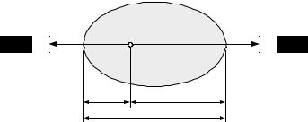
Consider the attenuation in an object whose total thickness is D, measured along the LoR, and the attenuation coefficient is µ, as shown in Fig. 2.7. If the annihilation event occurs at position x, measured along the LoR, then the probabilities for the two gamma rays to reach the opposing detectors are e−µ(D−x) and e−µx, respectively. The probability of registering the coincidence event is the product of the probabilities of detection of the gamma rays by the opposing detectors, i.e. e−µ(D−x) · e−µx ≡ e−µD , which is independent of the source position, x. This remains true when the attenuation coefficient is not uniform within the cross-section of the body. Thus, the attenuation is always the same even if the source position is outside the object.
The measured projection data will differ from the unattenuated projection data in the same fashion. Suppose µ(x, y) denotes the attenuation coefficient
Object
Detector |
Detector |
xD − x
D
Figure 2.7: Attenuation of the gamma rays in an object for a given line of
response.

Quantitative Functional Imaging with Positron Emission Tomography |
81 |
map of the object, the general equation for the attenuated projection data can
be described by the attenuated Radon transform
∞
pm(r, θ ) = f (x, y) exp − µ(x , y )ds dlr,θ (2.18)
0 0
where pm(r, θ ) is the measured projection data, l(x, y) is the distance from the detector to a point (x, y) in the object, while lr,θ and r have the same definitions as in equations (2.6) and (2.7). It should be noted that unlike the unattenuated Radon transform as in equation (2.6), there is no analytical inversion formula available for equation (2.18).
The attenuation correction in PET is simpler and easier as compared to SPECT due to the difference in the photon detection schemes. In SPECT, the attenuation depends not only on the source position, but also on the total path length that the photon travels through the object. It is not straightforward to correct for attenuation or find an inversion of equation (2.18) for image reconstruction. On the contrary, the attenuation in PET is independent of the source position because both gamma rays must escape from the body for external detection and the LoR can be determined. Therefore, the exponential term in equation (2.18) can be separated from the outer integral. The unattenuated projection data and the measured projection data can then be related as follows:
pm(r, θ ) = p(r, θ ) pµ(r, θ ) |
(2.19) |
|
where p(r, θ ) is the unattenuated projection data, and |
|
|
pµ(r, θ ) = exp − 0 |
∞ µ(x, y) dlr,θ |
(2.20) |
is the projection data of the attenuation map. Therefore, if the attenuation coefficient map µ(x, y) or its projection data pµ(r, θ ) is known, then the unattenuated projection data p(r, θ ) of the object can be calculated as:
pm(r, θ )
(2.21)
pµ(r, θ )
and f (x, y) can then be reconstructed without attenuation artifacts.
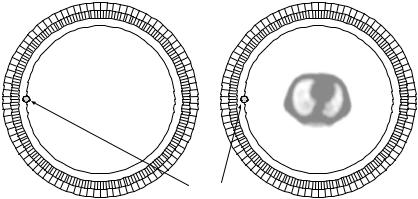
Since the attenuation is always the same regardless of the source position inside the FOV, it is possible to use an external (transmission) positron-emitting source that comprises a fixed ring or rotating rod sources, to measure the attenuation correction factors through two extra scans: blank scan and transmission scan. A blank scan is acquired with nothing inside the FOV, and a transmission
82 |
Wong |
Blank scan |
Transmission scan |
Patient
Ge-68 rotating rod source
Figure 2.8: Attenuation correction in PET using a rotating rod source of
68Ge. Blank and transmission scans are generally acquired before tracer administration.
scan is acquired to measure the coincidence rate when the patient being imaged is in the FOV but has not been given an injection of positron emitter. Figure 2.8 shows a schematic for measured attenuation correction using a rotating rod source of positron emitter 68Ge. Attenuation correction factors are then determined by calculating the pixelwise ratio of the measured projection data obtained from the blank scan and the transmission scan. The major drawback of this approach is that statistical noise in the transmission data would propagate into the emission images [46, 47]. Therefore, transmission scans of sufficiently long duration have to be acquired to limit the effect of noise propagation. Depending on the radioactivity present in the external radiation source and on the dimension and composition of the body, transmission scans of 15–30 min are performed to minimize the propagation of noise into the emission data through attenuation correction, at the expense of patient throughput. Further, lengthened scan duration increases the likelihood of patient movement, which can cause significant artifacts in the attenuation factors for particular LoRs.
Application of analytical, so-called calculated attenuation correction eliminates the need for a transmission scan, thus making this method attractive in many clinical PET centers. This method assumes uniform skull thickness and constant attenuation in the brain and skull. However, such assumptions
Quantitative Functional Imaging with Positron Emission Tomography |
83 |
do not hold for sections that pass through sinuses and regions where the adjacent bone is much thicker. Alternatively, the transmission scan may be performed after tracer administration, referred to as postinjection transmission (PIT) scanning [48], which utilizes strong rotating rod (or point) sources for the transmission source. A small fraction of “transmission” coincidences contains in the sinogram data can be distinguished from emission coincidences that originate from the administered radiopharmaceuticals by knowing the positions of the orbiting sources. Another approach is to integrate measured and calculated attenuation that makes use of the advantages of each approach. A transmission scan is still required and the attenuation coefficient images derived from the transmission and blank scans are reconstructed and then segmented into a small number of tissue types, which are assigned with a priori known attenuation coefficients [49–51]. These processes greatly reduce noise propagation from the transmission data into the reconstructed emission images.
2.12 Calibration
Once the acquired data has been corrected for various sources of bias introduced by different physical artifacts as mentioned in the previous section, images can be reconstructed without artifacts, provided that there are sufficient axial and angular sampling of projection data. To reconstruct images in absolute units of radioactivity concentration (kiloBecquerel per milliliter, kBq/mL, or nanoCurie per milliliter, nCi/mL), calibration of the scanner against a source of known activity is required. This can be accomplished by scanning a source of uniform radioactivity concentration (e.g. a uniform cylinder) and then counting an aliquot taken from the source in a calibrated well-counter to obtain the absolute activity concentration, which is then compared to the voxel values in the reconstructed images for the source (after corrections for physical artifacts have been applied) to determine a calibration factor.
2.13 Resolution Limitations of PET
Although there has been significant improvement in PET instrumentation over the last two decades, there is a finite limit to the spatial resolution of PET scanner.