Kluwer - Handbook of Biomedical Image Analysis Vol

[96]Tsui, E. and Budinger, T. F., Transverse section imaging of mean clearance times, Phys. Med. Biol., Vol. 23, pp. 644–653, 1978.

[97]Phelps, M. E., Mazziotta, J. C., and Huang, S. C., Study of cerebral function with positron computed tomography, J. Cereb. Blood Flow Metab., Vol. 2, pp. 113–162, 1982.

[98]Mazziotta, J. C. and Phelps, M. E., Positron emission tomography studies of the brain, In: Positron Emission Tomography and Autoradiography: Principles and Applications for the Brain and Heart, Phelps, M. E., Mazziotta, J. C., and Schelbert, H. R., eds., Raven Press, New York, pp. 493–579, 1986.

[99]Grafton, S. T. and Mazziotta, J. C., Cerebral pathophysiology evaluated with positron emission tomography, In: Diseases of the Nervous System: Clinical Neurobiology, Asbury, A. K., Mckhann, G. M., and McDonald, W. I., eds., Saunders, Philadelphia, pp. 1573–1588, 1992.

[100]Frey, K. A., PET studies of neurochemical systems, In: Positron Emission Tomography: Basic Science and Clinical Practice, Valk, P. E., Bailey, D. L., Townsend, D. W., and Maisey, M. N., eds., Springer, London, pp. 309–327, 2003.

[101]Bar-Shalom, R., Valdivia, A. Y., and Blaufox, M. D., PET imaging in oncology, Semin. Nucl. Med., Vol. 30, pp. 150–185, 2000.

[102]Rhodes, C. G., Wise, R. J., Gibbs, J. M., Frackowiak, R. J., Hatazawa, J., Palmer, A. J., Thomas, D. G. T., and Jones, T., Invivo disturbance of the oxidative metabolism of glucose in human cerebral gliomas, Ann. Neurol., Vol. 14, pp. 614–626, 1983.

[103] Di Chiro, G., Positron emission tomography using [18F]fluorodeoxyglucose in brain tumors: a powerful diagnostic and prognostic tool, Invest. Radiol., Vol. 22, pp. 360–371, 1987.

[104]Doyle, W. K., Budinger, T. F., Valk, P. E., Levin, V. A., and Gutin, P. H., Differentiation of cerebral radiation necrosis from tumor recurrence by [18F]FDG and 82Rb positron emission tomography, J. Comput. Assist. Tomogr., Vol. 11, pp. 563–570, 1987.

[105]Strauss, L. G. and Conti, P. S., The applications of PET in clinical oncology, J. Nucl. Med., Vol. 32, pp. 623–648, 1991.

[106]Glasby, J. A., Hawkins, R. A., Hoh, C. K., and Phelps, M. E., Use of positron emission tomography in oncology, Oncology, Vol. 7, pp. 41– 46, 1993.

[107]Coleman, R. E., Clinical PET in oncology, Clin. Pos. Imaging, Vol. 1, pp. 15–30, 1998.

[108]Anger, H. O., Scintillation camera, Rev. Sci. Instrum., Vol. 29, pp. 27–33, 1958.

[109]Smith, A. M., Gullberg, G. T., Christian, P. E., and Datz, F. L., Kinetic modeling of teboroxime using dynamic SPECT imaging of a canine model, J. Nucl. Med., Vol. 35, pp. 484–495, 1994.

[110]Smith, A. M., Gullberg, G. T., and Christian, P. E., Experimental verification of technetium 99m-labeled teboroxime kinetic parameters in the myocardium with dynamic single-photon emission computed tomography: Reproducibility, correlation to flow, and susceptibility to extravascular contamination, J. Nucl. Cardiol., Vol. 3, pp. 130–142, 1996.

[111]Iida, H. and Eberl, S., Quantitative assessment of regional myocardial blood flow with thallium-201 and SPECT, J. Nucl. Cardiol., Vol. 5, pp. 313–331, 1998.

[112] Eberl, S., Quantitative Physiological Parameter Estimation from Dynamic Single Photon Emission Computed Tomography (SPECT), Ph.D. Thesis, University of New South Wales, Australia, 2000.

[113]Laruelle, M., Baldwin, R. M., Rattner, Z., Al-Tikriti, M. S., Zea-Ponce, Y., Zoghbi, S. S., Charney, D. S., Price, J. C., Frost, J. J., Hoffer, P. B., and Innis, R. B., SPECT quantification of [123I]iomazenil binding to benzodiazepine receptors in nonhuman primates. I: Kinetic modeling of single bolus experiments, J. Cereb. Blood Flow Metab., Vol. 14, pp. 439–452, 1994.

[114]Boundy, K. L., Rowe, C. C., Black, A. B., Kitchener, M. I., Barnden, L. R., Sebben, R., Kassiou, M., Katsifis, A., and Lambrecht, R. M., Localization of temporal lobe epileptic foci with iodine-123 iododexetimide cholinergic neuroreceptor single-photon emission computed tomography, Neurology, Vol. 47, pp. 1015–1020, 1996.

[115]Chefer, S. I., Horti, A. G., Lee, K. S., Koren, A. O., Jones, D. W., Gorey,

J.G., Links, J. M., Mukhin, A. G., Weinberger, D. R., and London,

E.D., In vivo imaging of brain nicotinic acetylcholine receptors with 5-[123I]iodo-A-85380 using single photon emission computed tomography, Life Sci., Vol. 63, pp. PL355–PL360, 1998.

[116]Kassiou, M., Eberl, S., Meikle, S. R., Birrell, A., Constable, C., Fulham,

M.J., Wong, D. F., and Musachio, J. L., Invivo imaging of nicotinic receptor upregulation following chronic (-)-nicotine treatment in baboon using SPECT, Nucl. Med. Biol., Vol. 28, pp. 165–175, 2001.

[117]Pelizzari, C. A., Chen, G. T. Y., Spelbring, D. R., Weichselbaum, R. R., and Chen, C. T., Accurate three-dimensional registration of CT, PET and/or MR images of the brain, J. Comput. Assist. Tomogr., Vol. 13, pp. 20–26, 1989.

[118]Woods, R. P., Mazziotta, J. C., and Cherry, S. R., MRI-PET registration with automated algorithm, J. Comput. Assist. Tomogr., Vol. 17, pp. 536–546, 1993.

[119]Wagner, H. N., Jr., Images of the future, J. Nucl. Med., Vol. 19, pp. 599–605, 1978.

[120]Beyer, T., Townsend, D. W., Brun, T., Kinahan, P. E., Charron, M., Roddy, R., Jerin, J., Young, J., Byars, L., and Nutt, R., A combined PET/CT scanner for clinical oncology, J. Nucl. Med., Vol. 41, pp. 1369–1379, 2000.

where γ is gyromagnetic ratio, B0 is magnetic field strength, x, y, z are position vectors of a spin isochromat, and G is the applied gradient field vector. This vector has components viz. Gx, G y, and Gz along the x, y, and z directions, respectively. Inside the vessels, slight variations in magnetic field make the spin isochromats precess at different speeds. The spin isochromat precessing in different directions can be represented as different points on a precession circle. Simultaneously, they lose phase coherence in this process that results in loss of MR signal. However, two methods are commonly used to recover MR signal loss viz. refocusing 180◦ RF pulse and gradient recalled echo (GRE). Spin isochromat magnetization is inverted by applying excitation time less than TE i.e. T =

TE/2. Refocusing 180◦ RF pulse in spin echo (SE) sequence sent after time T =

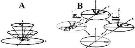
TE/2 inverts isochromat magnetization. The refocusing 180◦ RF pulse creates a head start. So, it refocuses the slow moving spins to reach the x axis as shown in Fig. 3.1. This whole process is known as dephasing or defocusing.

Figure 3.1: RF pulse is shown to flip the magnetization out of its orientation along the z-axis by a variable flip angle θ , magnetetization vector starts to precess, describing a isochromat circle in the x,y plane (Figure A) for spin-echo imaging at flip angle 90◦. After 90 pulse, the isochromats precess with different Larmor frequencies due to experience of different magnetic fields (shown with arrows). A typical spin-echo pulse is shown with RF pulse flipping magnetization 180◦ and back to create an echo (middle row). In GRE sequence, inverted readout gradient is used to invert precession and result refocusing pulse.

Alternatively, the gradient field-recalled echo or gradient inversion method inverts the precession direction of spin isochromats. Interestingly, sliceselection gradient is not needed after initial phase in this process. So, refocusing is achieved by using a negative read-out gradient for the first echo, a positive one for the second echo, and so on. In both methods, all the precessing isochromats point along the x direction after time TE. It results in first spin echo generation.

3.1.1.1 Spin Isochromats in Motion

Let us consider the case of time-dependent position x(t) of a spin isochromat in motion. The position may be represented as Taylor series expansion in the x direction:

x(t) = S + Vt + Axt2 + higher order terms

where S is initial position of spin isochromat, V is velocity, and A is acceleration in time t.

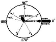
For simplicity, assume a spin isochromat moves along the x axis (y axis and z axis assumed zero) and read-out occurs along the x axis. In that case, according to Eq. (3.1), Gx gradient will have an effect on spin isochromat to generate precession phase of moving spin isochromat relative to stationary spin isochromat (see Fig. 3.2). This precession phase can be represented as

Figure 3.2: Precessing isochromats are shown in motion to result nonzero phase angle at odd echoes (arrows with lebel “0”). The isochromat magnetization vectors within a voxel add up to a small resultant vector (short thick arrow) if the isochromats within the voxel have different velocities. On even echoes, all isochromat magnetization vectors point in the 0◦ direction (along the x-axis) independent of velocity (arrows lebeled “e”).

The phases of precession and motion under the influence of gradient Gx may be explained to generate spin echo and even echo refocusing phenomena. Gradient field Gx is turned on. Precession phase of moving spin isochromat is integrated over different time intervals on a precession circle. It will show stationary spin isochromat pointing along the x direction at the first echo. Moving spin isochromats will point in any direction in the xy plane. Let us consider the basis of ‘even echo refocusing phenomenon’ in these spin isochromats. The phase angle in these spin isochromats is proportional to the velocity and gradient field strength Gx. However, the second and other even echoes (n = 2, 4, 6, . . .) have phase angle zero. The phase angles of even echoes are independent of velocity in the case of constant-velocity motion and symmetrical echoes.

These concepts explain the behavior of phase and motion. Variations in phase and motion of flowing blood inside vessels appear with variable spin-phase appearance of flowing blood. Similarly for accelerated motion, the phase angle is proportional to acceleration. In this case, even echo refocusing does not happen. Interestingly, velocity-induced phase changes are proportional to the time tp. tp is defined as the time during which the gradient field Gx is switched on, and is a function of the echo time (T = TE/2). Acceleration-induced phase changes are functions of the echo time TE and tp.

3.1.1.2 Flow Information in Spin Isochromats

In spin echo pulse sequence, gradient vectors are represented in the x, y, and z directions as Gx, G y, and Gz gradient fields. In an earlier section, motion in the gradient field Gx was explained. Let us consider the case of motion along the other gradient fields G y and Gz. Similar spin isochromat effects and relationship may be explained. These flow effects are stronger along the slice-selected gradient. These flow effects are negligible along phase encoding gradient. For read gradient, area under Gz, before and after 180◦ refocusing pulse are equal. On the contrary, for GRE sequence, read gradient is opposite. This read gradient is equal to 1, just prior to read-out gradient. So, the refocusing effect is generated. For it, during read-out, gradient is turned on for twice as long as that at the beginning of the pulse sequence.

Motion inside the vessels produces predictable changes in the precession phases of moving spin isochromats relative to stationary spin isochromats. Inside the vessel, for each voxel, phase angles can be determined based on the projections of magnetization Mxy along the x and y axes. Precessing spins in the voxel exhibit different phase angles. These phase angles in the voxel generate real and imaginary images. In general, the images may be represented as modulus or amplitude images in different voxels. These phase image amplitudes correspond to the length of magnetization vector Mxy. So, these images represent voxel-by-voxel velocity for applied gradient fields. In other words, motion can be identified as areas on phase images where phase is nonzero. However, in the voxel, spin phases and image generation suffer from magnetic field inhomogeneity artifacts. These inhomogeneity artifacts affect the entire magnetic field. An abrupt change in phase along a smaller intravascular area exhibits phase variation due to intravascular signal. This abrupt phase variation along a smaller area is used for generating image flow abnormality.

3.1.1.3Laminar, Turbulent and Pulsatile Flow in Human Vascular System

Blood flows in a human body in a well-defined physiological closed circulatory system. The flow is regulated by the heart and exhibits different flow properties known as flow patterns. Blood flow patterns are different at different locations in the intravascular system. MR signal intensities from such intravascular locations in cardiovascular and cerebrovascular systems appear dependent on hemodynamic properties of the cardiovascular or cerebrovascular system. The other important property of vascular system is flow velocity. In general, blood velocity inside a vessel is the largest at the center and zero around the walls. The flow velocity and vessel diameter plots are known as flow profile. This concept is significant in the analysis of MR signal loss.

Three types of flow velocities are representative viz. laminar, turbulent, and pulsatile flow (see Fig. 3.3). Laminar flow is defined as a flow pattern in which adjacent layers of fluid glide past each other without mixing different flowing blood layers. This type of flow may be called parabolic flow. The velocity varies quadratically with the distance from the center of the vessel. At the center, the

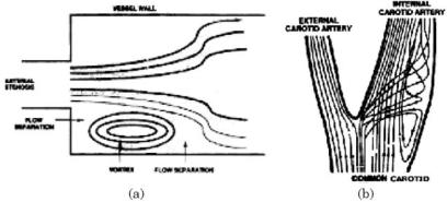
Figure 3.3: The central streamline flow separating from the vessel wall to produce a vertex or flow eddy stagnant blood to cause hemodynamic condition in VMRI (on left). The flow pattern at carotid bifurcation shows countercurrent flow and flow separation phenomena within the carotid bifurcation.

flow is maximum. Turbulent flow is defined as a rectangular flow pattern. The flow velocity is high in the whole region and vortices do appear. Adjacent layers are mixed. The flow is known as ‘plug flow’ otherwise velocity as a function of spin position is defined by Laminar flow as following:

where a is radius of vessel as cylinder. So, the plug flow for every phase-encoding step may be defined at constant flow as:

where G0 is bipolar pulse strength and τ is length of time and phase is γ Gvτ 2 with flow along x. In case of velocity as function of spin position for the flow along x when vessel is in-plane the laminar flow may be defined as:

These flow characteristics are interrelated by Reynolds number, Re, as:

where ρ is density and η is viscosity of fluid.

For Re > 2000, the flow is defined as turbulent flow. For Re > 7000, the flow is defined as pulsatile flow as observed in arteries for a transition state between

laminar and turbulent flow. First, laminar flow facilitates the acceleration of the blood flow to reach peak flow velocity. Later, the transition from laminar flow to turbulent flow appears as early phase in the deceleration phase soon after the peak velocity. In such situations, the transition flow depends upon the curvature and radius of a vessel. This flow generates forces parallel to the vessel wall termed as ‘shear force’. For example, shear forces are common at the points of atherosclerotic plaque in the arterial wall. The shear force can be represented as: s = ηδv/δr where η is coefficient of viscosity and δv/δr is the radial variation of velocity in the vessel. In the vessel, the shear force is greater close to the vessel wall. The reason for this is that the radial spatial variation in velocity is largest there.

In humans, laminar flow is common in veins and capillaries. This flow varies due to respiratory motion and arterial contractions. The flow velocity in the veins varies on the order of 10–20 cm/sec. In the arteries, blood flow is pulsatile with Reynolds number > 7000. In blood vessels, turbulence is rarely observed. However, turbulence may be seen in large arteries and systolic motion in the heart. Typical flow velocities in large arteries vary from zero in the end-diastolic phase of cardiac cycle to 50–100 cm/sec in the mid-systole. Larger spatial variations in flow velocity are also observed at the vessel walls near vascular bifurcation sites at which atherosclerotic plaque appears. In arteries, blood flow in cardiac chambers is pulsatile because cardiac chambers are large open spaces. In these chambers, R0 is large and inflow and outflow of blood result in vertex formation and also in large spatial velocity variations. This flow characteristic is known as ‘cine ventriculography’. Vertex formation is related to rapid inflow and outflow of blood in the cardiac chambers. In the diastolic phase, little flow and small volume changes are observed as short-lived phase. This short-lived phase of cardiac cycle depends on the heart rate. These are common in patients with low heart rates. In these patients blood is approximately stagnant during late diastole, while systolic events are less affected by heart rate. At heartbeats above 70 beats per minute, patients show appearance of vortices and spatial variation in flow velocity in cardiac chamber. These spatial variations affect systole and diastole. On the other hand, microvascular circulation occurs at flow velocities 0.5–1.0 cm/sec and is pulsatile in the arterioles up to the precapillary sphincter. It is continuous in the capillaries and venules distal to it. Vessel walls experience high shear forces. Microcirculation vessels do form a network of vessels with changing orientation inside the vessel.