Kluwer - Handbook of Biomedical Image Analysis Vol

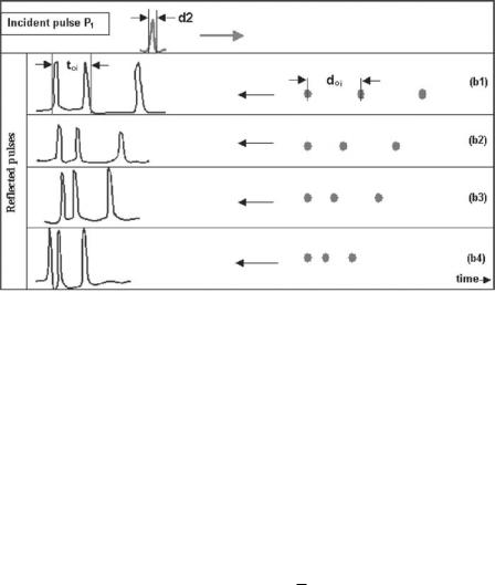
Figure 1.10: An ultrasound pulse P1 that has width d1 frontally affects a linear scatterer array placed at a distance doi.

transducers be smaller so that the resolution is increased, but this diminishes their capacity to explore greater tissues depth. For the IVUS techniques, the resolution plays a very important role since most of the structures to be visualized directly depend on these parameters.

1.4.1.1 Axial Resolution

Axial resolution is the capacity of an ultrasound technique to separate the spatial position of two consecutive scatterers through its corresponding echoes [13, 14, 16]. In Fig. 1.10 an ultrasound pulse P1 that has a width d1 frontally affects a linear scatterer array at a distance doi. Each one of the echoes forms a “train” of pulses temporally distanced according to the equation toi = 2|Ri|/c,

Ri being the ith relative emitter/scatterer distance and c is the pulse propagation speed. The progressive distance reduction of the linear scatterers, given by (a1, . . . , a4) (Fig. 1.10) and (b1, . . . , b4) (Fig. 1.11), reduces the time interval between the maximums of the “trains” pulses. There exists a critical distance width dt at which the pulses that arrive at the receiver are superposed, therefore, not being able to discriminate or separate individually the echoes produced by each scatterer. In Fig. 1.11 one can observe that the resolution can be improved by

Figure 1.11: We can see that the progressive distance reduction of the linear scatterers, from (a1, . . . , a4) (Fig. 1.10) to (b1, . . . , b4) reduces the time difference between the maximums of the “train” pulses. The maximums can be separated reducing the pulse width from d1 (Fig. 1.10) to d2, this is equivalent to an increase in the pulse frequency.

diminishing the pulse width dt , which is equivalent to increasing the frequency of the emitted pulse. The axial resolution of this technique depends essentially on two factors: ultrasound speed c and pulse duration dt . The functional dependency between the spatial resolution, the frequency, and the ultrasound speed propagation is given by:

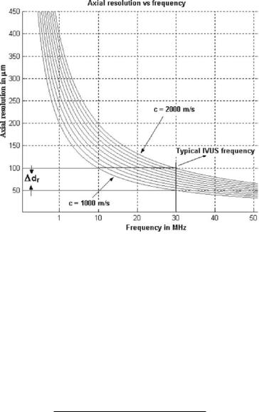
where dr is the axial resolution, c is the ultrasound speed for biological tissues, dt is the pulse width, T is the period of ultrasound wave, and f is the ultrasound frequency. For IVUS, the typical values are: c = 1540 m/sec and f = 30 MHz, the axial resolution is approximately dr = 1540/(30 × 106) = 0.05 mm ≈ 50 µm, and the relative error of the axial resolution is given by:

The axial resolution dependency versus the ultrasound frequency is shown in Fig. 1.12.

Figure 1.12: The functional dependency between the axial resolution and the ultrasound frequency for a rank of typical ultrasound speeds (see Table 1.1) in biological tissue. The typical IVUS (30 MHz) frequency as well as the tolerance in the axial resolution dr are emphasized.

1.4.1.2 Angular Resolution

Angular resolution is the capacity to discern two objects or events located in the tangential direction [13, 14, 16] and depends on the beam width. The beam

Table 1.1: Sound speed in selected

tissues [16]

where λ = c/ f and D is the transducer diameter. For a typical transducer of 30 MHz, c = 1540 m/sec and transducer dimensions given in Fig. 1.14, the lateral resolution is dθ ≈ 0.10◦ and the focal length is F = 2 mm.

1.4.2 The Beam Intensity

The beam ultrasound intensity, as a function of the penetration depth and the ultrasound frequency, is given by [13, 14, 16]:

where Io is the beam intensity at r = 0 and the coefficient α gives the rate of diminution of average power with respect to the distance along a transmission path [17]. It is composed of two parts, one (absorption) proportional to the frequency and the other (scattering) dependent on the particle size, or the scatterer number Nθ located along the ultrasound beam path (see Section 1.5.2). Since the attenuation is frequency dependent, a single attenuation coefficient only applies to a single frequency. The attenuation coefficient of ultrasound is measured in units of dB/cm, which is the logarithm of relative energy loss per centimeter traveled. In biological soft tissues, the ultrasound attenuation coefficient is roughly proportional to the ultrasound frequency (for the frequency range used in medical imaging). This means that the attenuation coefficient divided by the frequency (unit dB/MHz cm) is nearly constant in a given tissue. Typical soft tissue values are 0.5–1.0 dB/MHz cm. In our model we assumed that the attenuation coefficient α is only dependent on the scatterer number in the way beam. Figure 1.15 shows the beam intensity dependence on penetration depth for several typical frequencies used by IVUS.

1.4.3 Ultrasound Beam Sweeping Criterion

Let us explore a criterion that assures that all the reflected echoes reach the transducer before it moves to the following angular position. Let us define β as the ratio between transducer diameter D and arc length (Fig. 1.16):

β= D

where D is the transducer diameter and is the arc segment swept by the beam

diameters respectively, and a is the effective emission diameter of the transducer. Typical arterial lumen diameter of coronary arteries is D ≈ 3 mm [18,19]. From Fig. 1.14 we can see that DM ≈ 0.84 mm and a = 0.60 mm. Using Eq. (1.10) we obtain the sweeping volume of the transducer beam approximately as

Vb ≈ 3.91 mm3. The RBCs can be approximated by spherical scatterers having a volume of 87 µm3 [20], which corresponds to a radius of 2.75 µm (diameter, dg = 5.5 µm). Considering a typical hematocrit concentration [21] of 35%, we can estimate the RBCs number by the beam sweeping volume. The RBCs sweeping volume is VRBC = 1.36 mm3, and the typical human RBCs number is approximately N ≈ 4.1 × 106 cells/mm3 [21]. Thus, the RBCs number by the sweeping volume is No ≈ 5.61 × 106 cells. The maximal axial resolution at 40 MHz is approximately dr = 38 µm, at which we can observe the order of dr /dg ≈ 7 RBCs. If we take the scatterers as perfect spheres with radius dr at maximal axial resolution, we would have scatterers of the order of 1.37 × 107 to be simulated. It is not possible to estimate this value for RBCs scatterers with a computer. In order to generate the number of scatterers possible to emulate, we generate scatterers groups namely “voxel” [11]. In Table 1.2, the most important numerical data used by this simulation model is summarized. The minimal structure dimensions that can be measured by an IVUS image at 40 MHz is 1/25 mm/pixel ≈ 0.04 mm. We take this dimension to estimate the minimal

Table 1.2: Important features and the corresponding approximated values used in this simulation model

Nk is the scatterer number, Rk is the mean radial position, ηk is the radial deviation, µk is the backscattering cross section, and σk is the DBC deviation.

“voxel” volume. For the RBCs, Vo = 0.04 × 0.04 × 0.04 ≈ 6.4 × 10−5 mm3. The total number of RBCs per voxel is Nt = Vo × N ≈ 360 cells/voxel. Now, we can calculate the total RBCs “voxel” number as NRBC = No/Nt ≈ 1.5 × 104 voxels for the sweeping volume by the ultrasound beam. This “voxel” number is even computer intractable. Therefore, we must consider that the typical structure dimensions that can be measured by IVUS image are greater than 0.04 mm. A well contrasted image structure dimension by IVUS begins from 0.06 mm. Using these “voxel” dimensions, Vo = 2.14 × 10−4 mm3, the total “voxel” number is

Nt ≈ 880 cells/voxel, and the RBC “voxels” number is approximately N1 ≈ 6200 voxels. An example of RBCs “voxel” number used in this simulation is given in Table 1.3.

(2)The intima, media, and adventitia. The numerical values necessary for the evaluation of the scatterer number for the intima, media, and adventitia were taken from results of Perelman et al. [22], which give the typical nuclear cells size l (µm) distribution for human cells. The “voxel” number for each layer was computed taking into account the typical dimensions of intima, media, and adventitia of a normal artery.

(3)The voxel number for the sheathing transducer was calculated taking into account the minimal scatterers that can be observed at maximal resolution when the frequency is fixed at 40 MHz, a typical IVUS frequency. From Figs. 1.14

and 1.19, the transducer sweeping volume is Vt = π a(D2M − Dm2 )/4, where a ≈ 0.60 mm is the transducer diameter, and DM ≈ 0.84 mm and Dm ≈ 0.72 mm are the exterior and interior transducer sheathing diameters respectively. Using these dimensions, Vt ≈ 0.08 mm3. The sheathing “voxel” number No can be calculated as No = Vt / Vo, where Vt ≈ 0.08 mm3 is the sheathing volume by the beam and Vo = 4π dr3/3 is formed by the minimal spherical scatterers with radius