

Kluwer - Handbook of Biomedical Image Analysis Vol
.1.pdfA Basic Model for IVUS Image Simulation |
23 |
dr = c/ f able to be measured when the frequency f and the ultrasound speed c are known. Taken typical values for c = 1540 m/sec and frequency of 40 MHz,
Vo ≈ 2.39 × 10⁻⁴ mm3, thus No ≈ 370 “voxels.”
1.5 Simulation of IVUS Image
1.5.1 Generation of the Simulated Arterial Structure
Considering the goal of simulating different arterial structures, we can classify them into three groups: tissue structures, nontissue structures, and artifacts. The spatial distribution of the scatterer number with a given DBC, σ (R, , Z) at point (R, , Z), has the following contributions:
σ (R, , Z) = A(R) + B(R, , Z) + C(R) |
(1.11) |
where A(R), B(R, θ , Z), and C(R) are the contributions of tissue structures, nontissue structures, and artifacts respectively.
1.Tissue scatterers. These are determined by the contribution of the normal artery structures, corresponding to lumen, intima, media, and adventitia. Figure 1.20 shows a k-layers spatial distribution of the scatterers for a simulated arterial image. These scatterers are simulated as radial Gaussian
Figure 1.20: A plane of k-layers simulated artery. The scatterer numbers are
represented by the height coordinate in the figure.

24 |
Rosales and Radeva |
distributions [23] centered in the average radius Rk and having standard deviation ηk corresponding to each arterial structures. Tissue scatterers are represented by:
|
|
ak |
|
− |
(R − Rk)2 |
|
A(R) |
ko |
exp |
(1.12) |
|||
|
= k=1 ηk |
2ηk2 |
|
|||
where ak is the maximal number of scatterers at R = Rk, k is the kth radial simulated tissue layer, and Rk is the radial layer average position.
2.Nontissue scatterers. These contributions can be made by structures formed by spatial calcium accumulation, which are characterized as having greater DBC density than the rest of the arterial structures. They are simulated by a Gaussian distribution in the radial, angular, and longitudinal arterial positions of the simulated structure:
|
|
|
|
bl cmdn |
|
|
|
|
|
|
|
|
|||
|
|
lo |
mo no |
|
|
|
|
|
|
|
|
|
|||
B(R, , Z) = l=1 m=1 n=1 |
βl γmνn |
F(R, , Z) |
|
|
|
|
|||||||||
|
= |
|
− 2 |
|
βl2 |
+ |
γm2 |
|
+ |
|
νn2 |
||||
F(R, , Z) |
|
exp |
|
1 |
|
(R − R |
l )2 |
|
( − |
m)2 |
|
|
(Z − Zn)2 |
|
|
|
|
|
|
|
|
|
|
|
|
|
|||||
where (l, m, n) correspond to the radial, angular, and longitudinal axes directions, (lo, mo, no) are the structures number in radial, angular, and longitudinal directions, (bl , cm, dn) are the scatterer numbers that have a maximum at R = Rl , = m, and Z = Zn, (βl , γm, νn) are the radial, angular, and longitudinal standard deviations, and (Rl , m, Zn) are the radial, angular, and longitudinal average positions.
3.Artifacts scatterers. In our model we consider the artifact caused by the sheathing transducer:
|
= |
αo |
− |
2αo2 |
|
||
C(R) |
|
|
ao |
exp |
|
(R − Ro)2 |
|
|
|
|
|
|
|
||
where ao is the scatterers number that has a maximum at R = Ro, αo is the artifact standard deviation, and Ro is the artifact radial average position.
1.5.2 1D Echogram Generation
To obtain a 1D echogram, an ultrasound pulse is generated in accordance with Eq. (1.4) and emitted from the transducer position. The pulse moves
A Basic Model for IVUS Image Simulation |
25 |
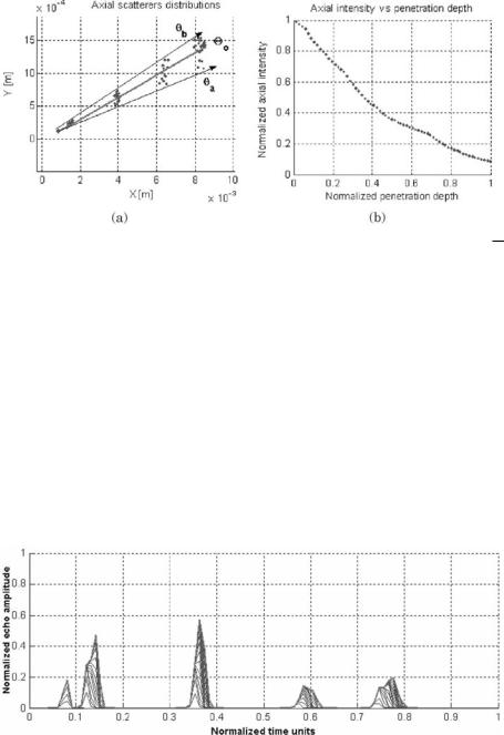
Figure 1.21: The 1D echogram is obtained by fixing the angular position 0 =
of the ultrasound beam (a). The total signal S(t) is only generated by the scatterers N located at an angular position a ≤ 0 ≤ b. The intensity distribution decreases with the depth penetration and the scatterers numbers N through the beam path (b).
axially through scatterers (Fig. 1.21(a)) and its intensity distribution decreases (Fig. 1.21(b)) with the penetration depth and the scatterers numbers in the ultrasound path given by Eq. (1.8). The echo amplitude is registered by the transducers (Fig. 1.22) as a signal function of time S(t) (Eq. 1.13). The value is transformed to penetration depth replacing t = x/c and normalized to gray scale. The spatial distribution of cross-section scatterers, σ , is generated by
Figure 1.22: The corresponding echoes are finally transformed to normalized echo amplitude and then to gray-level scale versus time or penetration depth.
26 |
Rosales and Radeva |
using Eq. (1.11). Figure 1.21 shows the simulations of N scatterers located in (Ri, a ≤ j ≤ b):
S(t, ) |
|
NR |
N i |
σ (Ri, o ± j )ζ (t, δi) |
|
|
|
(1.13) |
||||||||
|
|
|
|
|
|
|
|
|
|
|
|
|
||||
o |
|
= i |
|
1 |
j |
1 |
|
|
|Ri| |
|
|
|
|
|||
|
|
= |
= |
|
= |
|
|
|
|Ri| |
− |
2σ 2 |
|
− i |
|||
o |
) |
C |
o |
i=1 j=1 |
||||||||||||
S(t, |
|
|
|
NR |
|
Nθi |
σ (Ri, o ± j ) exp |
|
(t − δi)2 |
sin(ωt |
δ ) |
|||||
|
|
|
|
|
|
|
|
|
|
|
|
|
||||
where o = ( a + b)/2, Co defines the transducer constant parameters, and
N i is the total scatterers number at the angular position θa ≤ ≤ θb for a radial position Ri. The sum only operates on the scatterers located in the angular position θa ≤ ≤ θb that is the focal transducer zone (Figs. 1.9(b) and 1.13). Therefore, N is the total scatterers number in this region. Equation (1.13) can be written as a function of the penetration depth, replacing t = x/c. Equation (1.13) can be rewritten on gray-level scale as:
|
|
|
|
|
|
|
N |
Nθ |
|
|
|
|
|
|
|
|
|
|
256 |
|
|
|
|
σ (Ri, o ± j ) |
|
|
|
(t − δi)2 |
|
|
|
||
S(t, |
) |
|
|
|
C |
|
|
|
|
exp |
|
|
|
sin(ωt |
|
δ ) |
o |
|
= max(S(t)) |
|
o |
i=1 |
j=1 |
|Ri| |
− |
2σ 2 |
|
− |
i |
||||
(1.14) where δi = 2Ri/c and S(x) is the 1D echogram generated by a set of N scatterers located in (Ri, a ≤ i ≤ b). The overall distribution backscattering crosssection σi(Ri, i ± δ ) is given by Eq. (1.11).
1.5.3 2D Echogram Generation
The procedure to obtain the 2D simulated IVUS is the following: A rotatory transducer with angular velocity ω (Fig. 1.23(a)) is located at the center of the simulated arterial configuration given by Eq. (1.11). The transducer emits an ultrasound pulse radially focused at frequency fo along angular direction
θ1 (Fig. 1.23(a)). The pulse progressively penetrates each one of the layers of the simulated arterial structure according to Eq. (1.15). Each one of the layers generates a profile of amplitude or echoes in time, which can be transformed into a profile of amplitude as a function of the penetration depth (Fig. 1.23(b)). Therefore, the depth can be calculated using Eq. (1.1). As the penetration depth is coincident with the axial beam direction, the radial coordinate R is thus determined. This procedure is repeated n times for angles, (θ1, . . . , θn) and the 2D image is generated. The generated echo profiles are transformed to a polar

A Basic Model for IVUS Image Simulation |
27 |
Figure 1.23: The transducer emits from the artery center (a), echo profile transformed into penetration depth (b), the echo profiles are transformed to a polar image (c), and empty pixels filled and the final IVUS image is smoothed (d).
image, and the intermediate beams are computed (Fig. 1.23(c)). The image is transformed to Cartesian form and the empty pixels are filled (Fig. 1.23(d)).
Using the ultrasound reflected signal S(t, ) for a finite set of N reflecting scatterers with coordinates (R, , Z) and spatial distribution of the differential backscattering cross-section, σ (R, , Z), the 2D echo signal S(t, ) can be written as:
S(t, ) |
C |
|
NR |
Nθi |
σ (Ri, ± θ j )ζ (t, δi) |
(1.15) |
|
= |
|
o |
|
|
|
||
|
i 1 |
j |
1 |
|Ri| |
|
||
|
|
|
= |
= |
|
|
|
where S(t, ) is the temporally generated signal by a set NR of scatterers, which are localized in angular position θ , θ [θa, θb], Nθi is the total scatterers number

28 |
Rosales and Radeva |
in the angular position θa ≤ ≤ θb for a radial position Ri. We consider two
forms of :
with no uniform distributed scatterers:
= (θa + θb)/2
with uniform distributed scatterers:
= 1 NR j NR j=1
1.5.4 Final Image Processing
The actual image obtained with only the original beams is very poor; we must explore several smoothing procedures to improve the image appearance. The procedures to obtain the final simulated image are as follows:
1. The echoes are obtained by the pivoting transducer (Fig. 1.23(a)).
2. Each echo profile is ordered according to the angular position (Fig. 1.23(b)).
3.The original image is transformed to a polar form (Fig. 1.23(c)).
4.Secondary beams are computed between two original neighboring beams (Fig. 1.23(c)).
5.The image is smoothed by a 2 × 2 median filter.
6.The image is again transformed to Cartesian form. As a result of this transformation, a significant number of pixels will be empty (Fig. 1.23(d)).
7.The empty pixels are filled in a recursive way form, using an average of the eight nearest neighbors (Fig. 1.23(d)).
8.An image reference reticle is added and a Gaussian filter is applied.
Figure 1.24 shows the scatterers distribution for a concentric arterial structure and an axial ultrasound beam position (a), and its corresponding echo profiles
(b). Each axial echo is positioned by an angular position (c). In this way, the 2D echogram is constructed (d). The procedure of image smoothing is described in Section 1.5.4.

A Basic Model for IVUS Image Simulation |
29 |
Figure 1.24: The scatterers distribution (a), the corresponding 1D echoes (b), 2D echogram is constructed (c), and the image is smoothed (d).
1.6 Validation of the Image Simulation Model
Once the generic basic model of IVUS image formation is defined, we need to compare it to real images contrasting expert opinion to test its use. For this purpose, we defined procedures to extract quantitative parameters that permit the measurement of the global and local similarities of the images obtained. The main goal of this simulation is to give a general representation of the principal characteristics of the image. The comparison of real and simulated images should be done on the global image descriptors. We concentrated on the distribution of the gray levels. Data such as transducer dimensions (Fig. 1.14), the catheter as well as the reticle locations, operation frequency, band width,

30 |
Rosales and Radeva |
and original and secondary beam number used for the simulation are standard values obtained from Boston Sci. [24]. However, the optimal values of frequency and attenuation coefficient are obtained by the cross validation procedure [23]. The dimensions, scatterer number, and the backscattering crosssection of the simulated arterial structures were obtained from different literature [7, 10, 11, 19, 22, 24]. Typical values of the RBCs “voxel” numbers took into account the typical hematocrit percentage [11] (Section 1.4.4). Instrumental and video noise has been incorporated into the simulated image, due to electronics acquisition data, and the acquisition and processing to the video format.
The zones of greater medical interest (lumen, lumen/intima, intima/media, and media/adventitia) were simulated for several real IVUS images. The smoothing image protocol is not known so that the corresponding tests were done until the maximal similarity to the real images was found, based on the use of three progressive methods. (1) The empty pixels are filled using the average of eight neighbors, (2) a median filter is used, and (3) a Gaussian filter is applied in order to find the noise reduction. The quantitative parameters used for the image comparison were directed for global and local image regions, and are described below.
1.Gray-level average projections px and py, that is horizontal and vertical image projections, are defined for an m × n image I as [25]:
|
|
|
|
|
|
|
|
|
1 |
m |
|
1 |
n |
|
|
||
px(i) = |
m |
j=1 |
Iij , |
py( j) = |
n |
i=1 |
Iij |
(1.16) |
2.We define a global linear correlation between real (x) and simulated (y) data as follows:
y = mx + b |
(1.17) |
where m and b are the linear correlation coefficients.
3. Contrast to noise ratio signal (CNRS) as figure of merit, defined as [26]:
(µ1 − µ2)2
CNRS = (1.18)
σ12 + σ22
where µ1, µ2, σ1, and σ2 are the mean and the standard deviations inside
the ROIs.
A Basic Model for IVUS Image Simulation |
31 |
1.6.1 Scatterer Radial Distribution
The radial scatterer distribution is an important factor for a good image simulation. The scatterers under consideration in this simulation are: the transducer sheath, blood, intima, media, and adventitia. We can obtain the arterial structure configuration from an emulated form and from a real validated IVUS image. For the study of the synthetic images, we have used two procedures:
1.Standard data. Typical geometric arterial parameters and their interfaces such as lumen/intima, intima/media, and media/adventitia are obtained from standard literature.
2.Validated data. Geometrical parameters are obtained from manually segmented IVUS images.
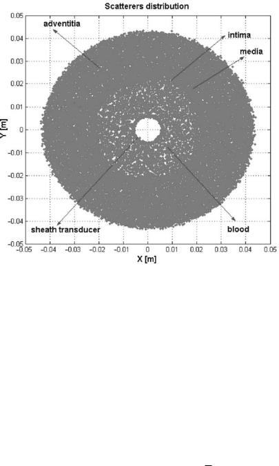
In order to investigate the image dependencies of IVUS parameters (frequency, attenuation coefficient, original beam number, secondary beam, and smoothing procedures), we have used a standard data procedure, using a concentric scatterer distribution for this modality. To compare simulated images to real data, we use manually segmented real images, which correspond to the validated data procedure. In manually delineated structures of IVUS images, we extract the position radius Rk of lumen, intima, media adventitia, and transducer sheath. Figure 1.25 shows typical 2D spatial scatterer distributions obtained from standard procedure for the most important arterial structures and the scatterer artifact caused by the transducer sheath.
The radial scatterer distributions play a crucial role in the definition of the IVUS images because they define the ultrasound attenuation in the axial direction. Medical doctors have special interest in gray-level transition in the interface of two media. For instance, the lumen/intima transition defines the frontiers of the lumen. These transitions can only be found through a good radial scatterer distribution.
The radial scatterers distribution of the typical arterial structures and the transducer sheath are shown in Fig. 1.26.
1.6.2 DBC Distribution
The k-layers DBCk values for a typical simulated arterial structure are shown in Figs. 1.27 and 1.28 where the count of scatterers of each tissue is shown as
32 |
Rosales and Radeva |
Figure 1.25: Typical concentric 2D scatterer distribution for the most important simulated arterial structures (blood, intima, media, and adventitia) and the scatterer artefact generated by the transducer sheath.
a function of the cross-section of scatterers. The numerical values are given in Table 1.3 [27].
1.6.3 IVUS Image Features
1.6.3.1 Spatial Resolution
A good spatial resolution gives the possibility of improving the visualization of the lumen/intima transition and studying the structures, which gives important information for medical doctors. Typical numerical parameters such as
scatterers number Nk, k-layer average radial position Rk, its standard deviation ηk, the DBC k-layer mean µk, and its standard deviation σk are given in Table 1.3. The typical IVUS parameters used in this simulation are given in