

Kluwer - Handbook of Biomedical Image Analysis Vol
.1.pdfA Basic Model for IVUS Image Simulation |
33 |
Figure 1.26: Radial scatterer distribution for the arterial structure: blood, intima, media, adventitia, and the transducer sheath.
Figure 1.27: DBC distributions of simulated arterial structures: blood (a) and
intima (b).
34 |
Rosales and Radeva |
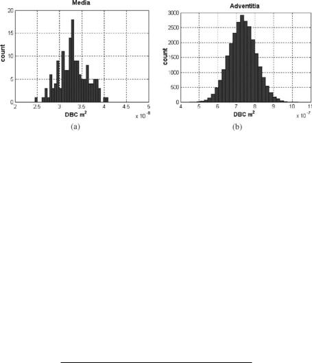
Figure 1.28: DBC distributions of simulated arterial structures: media (a) and adventitia (b).
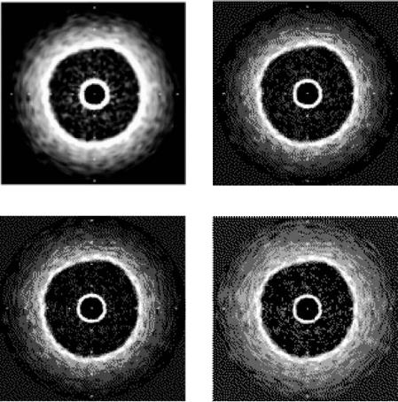
Table 1.4. The typical cell nuclear size was obtained by Perelman et al. [22]. In Fig. 1.29 we can observe the dependency of axial resolution and the ultrasound frequency. To illustrate this, four IVUS simulated images are shown. Low frequency ranging from 10 to 20 MHz corresponds to an axial resolution from 154 to 77 µm, and intermediate frequency from 20 to 30 MHz gives axial resolution from 77 to 51 µm. In these cases, it is possible to visualize accumulations around 100 RBCs. High frequency from 30 to 50 MHz leads to 51–31
µm of axial resolution. Moreover, it is now possible to visualize accumulations of tens of RBCs. The IVUS appearance improves when the frequency increases, allowing different structures and tissue transition interfaces to be better detected.
Table 1.4: Typical IVUS simulation magnitudes
Parameter |
Magnitude |
|
|
Ultrasound speed |
1540 m/sec |
Maximal penetration depth |
2E − 2 m |
Transducer angular velocity |
1800 rpm |
Transducer emission radius |
3E − 4 m |
Attenuation coefficient α |
0.8 dB/MHz cm |
Ultrasound frequency |
10–50 MHz |
Beam scan number |
160–400 |
Video noise |
8 gray level |
Instrumental noise |
12.8 gray level |
Beta parameter |
β = 38.5 ad |
A Basic Model for IVUS Image Simulation |
35 |
(a) |
(b) |
(c) |
(d) |
Figure 1.29: Synthetic images generated by low frequency: 10 MHz (a) and 20 MHz (b), intermediate frequency of 30 MHz (c), and high frequency of 50 MHz (d).
1.6.3.2 Optimal Ultrasound Frequency
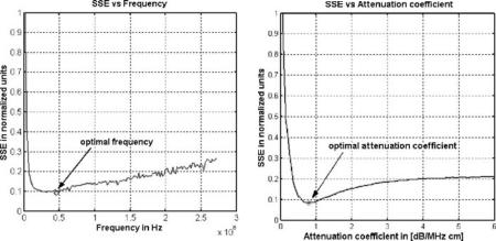
In order to validate our model, we compare synthetic to real images. We generated synthetic images for a great rank of frequency and used the cross-validation method [23] to find the most similar image to the real one generated using Boston Sci. equipment at 40 MHz frequency. The sum square error (SSE) from the real to the simulated images for each ultrasound simulated frequency is computed. Figure 1.30(a) shows the SSE versus ultrasound frequency. The optimal frequency
36 |
Rosales and Radeva |
(a) |
(b) |
Figure 1.30: The optimal ultrasound simulation frequency fo ≈ 46 MHz (a) and the optimal attenuation coefficient (b) α ≈ 0.8 dB/MHz cm are obtained by the cross validation method.
is located in the interval 40–50 MHz. Note that the central frequency of Boston Sci. equipment is 40 MHz; therefore, it can be considered as evidence to show the correctness of the method.
1.6.3.3 Optimal Attenuation Coefficient
We have emulated synthetic IVUS images with different attenuation coefficients; the optimal attenuation coefficient was tested by applying the cross validation method of the synthetic images versus the real images. Figure 1.30(b) shows SSE versus attenuation coefficient α; the optimal attenuation coefficient obtained was 0.8 dB/MHz cm. There is a range of suboptimal attenuation coefficient values for a fixed ultrasound frequency due to the great axial variability of scatterers. However, the attenuation coefficient can be taken as constant for each simulated region [28]; however, in the transition zones (lumen/intima, intima/media, and media/adventitia) the attenuation gives great variability. For this reason, we must average the attenuation coefficient value. It is very important to confirm that the optimal frequency is approximating the standard central ultrasound frequency of 40 MHz and that the attenuation coefficient is near the standard values of biological tissues, which ranges from 0.5 to 1 dB/MHz cm. This result can be used in different ways: first, to check the used simulation parameters in
A Basic Model for IVUS Image Simulation |
37 |
the case of ultrasound frequency and second to find structures of interest when the attenuation coefficient is known.
1.6.3.4 The Beam Number Influence
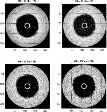
Figure 1.31 shows the appearance of several simulated IVUS images when the original and intermediate beam numbers are changed. We obtained the best appearance when the original beam number was 80 and the secondary beam number was 240. In total, 320 beams were used by the simulation. We can see that the IVUS appearance in the tangential direction is significantly affected by
(a) |
(b) |
(c) |
(d) |
Figure 1.31: Different combinations of original (NH) and intermediate (nh) beams yield different IVUS appearances.
38 |
Rosales and Radeva |
the beam number change. The total number of beams for the standard IVUS equipment is normally between 240 and 360 beams [24].
1.6.4 Real versus Simulated IVUS
In order to compare the real and simulated IVUS images, we have generated 20 synthetic images with morphological structures corresponding to the structures of a set of real images. We have used a real IVUS image with manually delimited
lumen, intima, and adventitia to obtain the average radius location Rk for each
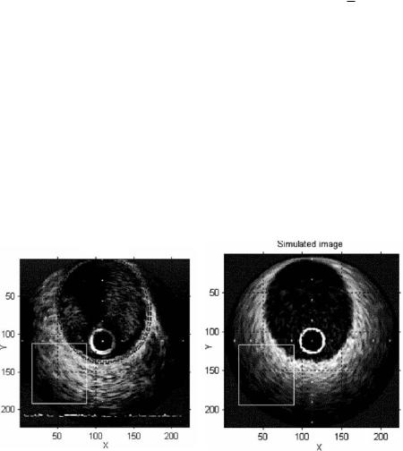
arterial structure. We applied the optimal frequency of 46 MHz and attenuation coefficient of 0.8 dB/MHZ cm. Figure 1.32(a) shows an IVUS real image of right coronary artery, obtained with a 40 MHz Boston Sci. equipment. Figure 1.32(b) shows a simulated image obtained at the optimal ultrasound simulation frequency of 46 MHz. In the real image, we can observe a guide zone artifact (12 to 1 o’clock) due to the presence of guide; this artifact will not be simulated in this study. The horizontal ECG baseline appears as an image artifact on the bottom of the real image. The global appearance of each image region (lumen, intima, media, and adventitia) and its corresponding interface transitions (lumen/intima, intima/media, and media/adventitia) are visually well contrasted, compared to the real image. A good quantitative global measure for comparison
Real image |
Simulated image |
|
(a) |
(b) |
Figure 1.32: Real (a) and simulated (b) IVUS images segmentation. ROIs are given as squares. Manual segmentation of the vessel is given in (a).
A Basic Model for IVUS Image Simulation |
39 |
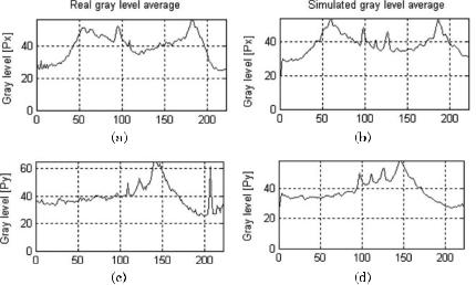
Figure 1.33: Horizontal ((a) and (b)) and vertical directions ((c) and (d)) gray-level profile average projections, from real (Fig. 1.32(a)) and simulated (Fig. 1.32(b)) IVUS images.
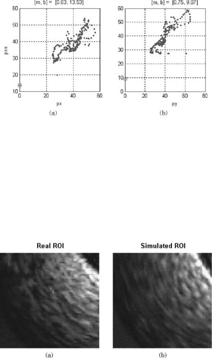
is the average gray-level projection that allows a simple form to find the main image correlated characteristics in an 1D shape gray-level profile. Gray-level baseline, video noise, instrumental noise, reticle influence, and the main graylevel distribution coming from the main arterial structures are roughly visible from the gray-level average projection. The average gray-level projection gives a global measure of the similarity between real and simulated images. The similarity measured can be computed, for example, by the local attenuation coefficient of the projection profile of each ROI [28]. Figure 1.33 gives the projections in the horizontal and vertical directions for the real (Fig. 1.32(a)) and simulated (Fig. 1.32(b)) IVUS images. The correlation coefficients mand b (Fig. 1.34) for the gray-level average projection in the horizontal (m = 0.63, b = 13.53) and vertical (m = 0.75, b = 9.07) directions show a positive correlation between the real and simulated data. Figure 1.35 shows two selected regions of interest of the real (Fig. 1.32(a)) and simulated (Fig. 1.32(b)) images. We can see a good gray-level distribution and a soft gray-level decay from the center to the peripheries of the IVUS image, produced by the inverse relation between the ultrasound intensity and the penetration depth. The other reason is that the normal attenuation is caused by the scattering intensity given by the tissue impedance. Figure 1.36
40 |
Rosales and Radeva |
Figure 1.34: Horizontal correlation using (a) versus (b) from Fig. 1.33 and the vertical global correlation using (c) versus (d) from the same figure.
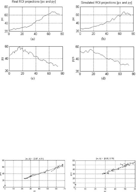
shows gray-level average projections in the vertical direction ((a) and (c)) and the horizontal direction ((b) and (d)) of the selected ROIs from Figs. 1.32(a) and (b). The linear correlation coefficients m and b (Fig. 1.37) for the gray-level average projection in the horizontal direction (m = 0.87, b = 4.91) and vertical direction (m = 0.85, b = 5.79) show a significant gray-level correspondence between the real and simulated ROIs image.
Figure 1.35: Real (a) and simulated (b) IVUS image ROIs.
A Basic Model for IVUS Image Simulation |
41 |
Figure 1.36: Horizontal ((a) and (b)) and vertical ((c) and (d)) projections of (Fig. 1.35(a)) and simulated (Fig. 1.35(b)) ROIs IVUS images.
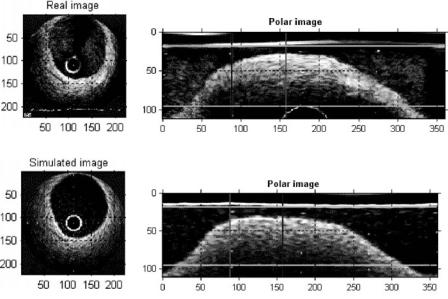
1.6.5 Polar Images
A polar representation of IVUS images offers several advantages: (1) The ROIs to study are very easy to select, (2) we can compare the artifact generated by the smoothing procedures, (3) radial and angular comparisons are totally separated, therefore the transition zones in each direction are very easy to observe. Figure 1.38 shows real (a) and simulated (c) Cartesian IVUS images and the corresponding real (b) and simulated (d) polar transformations. An ROI was selected
(a) |
(b) |
Figure 1.37: Gray-level average correlation, horizontal simulated (pxs) versus real projection (px), obtained from Fig. 1.36(a) versus (b), and vertical simulated (pys) versus real (py) data, from Fig. 1.36(c) versus (d).
42 |
Rosales and Radeva |
(a) |
(b) |
(c) |
(d) |
Figure 1.38: Real (a) and simulated (c) Cartesian images and their corresponding real (b) and simulated (d) polar transformation.
from the real and simulated polar images and the correlation coefficients were obtained. Figure 1.39(a) shows the gray-level average vertical projection for the real and simulated ROIs data (delineated in red in Fig. 1.38). We can see that the gray-level profiles of the transition of arterial structure in the lumen/intima, intima/media, and media/adventitia are very well simulated, the linear correlation coefficients being m = 0.93 and b = 1.61 (Fig. 1.39(b)). The global horizontal profile of the polar images along the projection θ (Figs. 1.40(a) and (b)) gives very important and comparative information about the real and simulated graylevel average of arterial structures. The information that can be extracted is relative to the global gray-level distribution. The histogram (Fig. 1.40(b)) of gray-level differences between the horizontal profiles of real and simulated data indicates a very good correspondence (mean µ = 8.5 and deviation σ = 10.2). Figure 1.41(a) shows the global projection in the radial direction (the vertical profile). We can see a very good correspondence between the gray-level shape profiles (mean µ = 5.7 and deviation σ = 8.5). The histogram (Fig. 1.41(b)) of gray-level difference confirms the good correlation between the real and simulated IVUS data.