Engineering and Manufacturing for Biotechnology - Marcel Hofman & Philippe Thonart

Macroscopic modelling of bioprocesses with a view to engineering applications

autocatalyse. A second kind of reaction is the catalytic reaction, e.g.

where is consumed, is produced and catalyses the reaction. This last

component is consumed and produced by the reaction, in the same quantity. It activates reaction (3) and is therefore necessary so that the reaction can occur. A third kind of

reaction consists of the autocatalytic reaction

where is consumed, is produced and autocatalyses the reaction. This latter

component is produced by the reaction. Moreover, it activates the reaction.

On the basis of the reaction scheme (1), the basic mathematical model structure is made of the mass balances for each of the macroscopic species

where

• is the vector of concentrations;

• is the dilution rate;

If the external substrates are diluted in the incoming culture medium, the corresponding components of the vector of external feed rates can be written

81

Ph. Bogaerts and R. Hanus

It may also happen that an external substrate is introduced in gaseous form (such as the oxygen in aerobic cultures). Then the corresponding component of the vector of external feed rates is given by

• is the saturation concentration.

By neglecting the dynamics of the liquid-gas transfer, the gaseous outflow rate of some component may be assumed to be proportional to the dissolved concentration:

where

Taking into account (6) and (8), the system (5) may be rewritten

where

• is the vector of concentrations in the components of the incoming stream;

• is a diagonal matrix containing the specific rates of liquid-gas transfer. Sufficient conditions of bounded input - bounded state (BIBS) stability have been

proposed in Bogaerts (1999) and in Bogaerts el al. (1999). The BIBS stability of a nonlinear differential system

(where x(t) is the state vector and u(t) is the input vector), guarantees that

82

Macroscopic modelling of bioprocesses with a view to engineering applications

i.e., that any bounded initial state x(0) and bounded input profile u(t) implies that the state trajectory x(t) remains bounded. Sufficient conditions of BIBS stability for the system of mass balances (9) can be summarised as follows.

2.1. FIRST SUFFICIENT CONDITION OF BIBS STABILITY OF (9)

A reference reactant for a given reaction is defined as a reactant which is neither a catalyst nor an autocatalyst and which is not produced in any other reaction of the scheme.

If

•the dilution rate is non negative (which is obvious from a physical point of view)

•the input concentrations are bounded

•each reaction of the scheme (1) contains at least one reference reactant

then

the states of the model (9) are positive and upper bounded for any time t.

2.2. SECOND SUFFICIENT CONDITION OF BIBS STABILITY OF (9)

If

•the dilution rate is non negative (which is obvious from a physical point of view)

•the input concentrations are bounded

•each reaction of the scheme (1), except reaction contains at least one reference

reactant;

provided reaction contains at least one reference reactant.

83

Ph. Bogaerts and R. Hanus

By taking the italic asserts away, the second condition reduces to the first one. The proofs of these sufficient conditions are sketched in Bogaerts et al. (1999) and detailed in Bogaerts (1999).

3. Kinetic model structure

3.1. MOTIVATIONS FOR A NEW KINETIC MODEL STRUCTURE

As shown in the previous section, the model structure consists of the mass balances (5) based on the reaction scheme (1). However, the structure of reaction rates contained in

concentrations The choice of these nonlinear functions is the matter of still ongoing

research.

We have already explained in the introduction why structured and/or segregated models will not be used in this formalism. They would lead to a significant increase in

components (or subpopulations of one component) to be measured. It could also lead, in some cases, to the impossibility of building engineering tools like software sensors (due to the unobservable feature of the model).

We have also recall the existence of some general mathematical modelling frameworks. The Biochemical System Theory (Savageau, 1969a, 1969b) uses power laws to describe the overall consumption and the overall production of each component. This kind of model can be linearised w.r.t. (with reference to) the parameters (thanks to a logarithmic transformation). This allows to benefit from the advantages of the linear parameter estimation, namely the existence, uniqueness and complete independence regarding any initial guess of the set of parameters which minimise a quadratic criterion (e.g., the least squares criterion). However, this property of the models in Biochemical System Theory is only available in steady state. Moreover, only the overall rates of consumption and production are given, without distinguishing the rates of a reaction scheme. Finally, BIBS stability and positiveness of the concentrations are not guaranteed a priori. Metabolic Control Analysis (Westerhoff and Kell, 1987) is a very structured approach with the drawbacks already mentioned before. Moreover the control coefficients and elasticity coefficients are not easy to determine. Cybernetic models (Dhurjati et al., 1985) seem to be difficult to apply in the (quite usual) case of a simultaneous consumption of several substrates. In order to reproduce the behaviour of such cultures, the structured part of the model has to be more complex (Ramakrishna et a/., 1996). Moreover the cybernetic approach seems not to be applicable with animal cell cultures (Tziampazis and Sambanis, 1994). Finally the general modelling methodology for animal cell cultures of Chotteau (1995) exhibits several problems like the computational load (several millions of solutions to be tested), the overall feature of the rate of consumption and/or production, the use of a black box polynomial model for

84

Macroscopic modelling of bioprocesses with a view to engineering applications

these overall rates (quasi without physical interpretation), the absence of guarantee for the BIBS stability of the model and for the concentration positiveness or, even, the possibility to simulate a spontaneous growth of living microorganisms (without any living cell present at the initial time of the experiment).

For all the above mentioned reasons, the existing general frameworks will not be used in the sequel and we will only focus on the remaining class of unstructured and unsegregated models which contains a large number of different structures. However, there are also several drawbacks exhibited by these solutions. First of all there is a lack of general structures. Indeed, there exist several Monod-type laws (see Appendix 1 of the book by Bastin and Dochain (1990) ), each one describing a limited number of physical effects (like the limitation and/or inhibition by substrate and/or biomass, etc.). Even for a given set of physical effects, there exist several solutions, e.g., the Monod, Tessier and Ming laws to describe the limitation of the specific growth rate by the substrate. Therefore a couple of questions arise: What set of physical effects must be chosen a priori ? For this set, what kind of law ? There is no systematic way to answer these questions. A second kind of problem, often linked to the solutions which are claimed to be more general, is the lack (or even absence) of physical meaning of the parameters. This is the case, for instance, with the artificial neural networks (Montague and Morris, 1994; Syu and Tsao, 1993) or with the general modelling methodology for animal cell cultures (Chotteau, 1995). A third problem is the absence of guarantee for the concentration positiveness, e.g., when using the famous Pirt law (Pirt, 1965) leading to a constant specific rate for the consumption of substrate linked to the maintenance. A fourth problem, occurring for instance in the methodology of Chotteau (1995), is the absence of guarantee of BIBS stability. Finally, a fifth disadvantage is that the models are nonlinear (which is necessary to reproduce the complex behaviour of bioprocesses) but, in most of the cases, non-linearisable w.r.t. the parameters, although this possibility is of great interest for the parameter identification problem (as stated above concerning Biochemical System Theory).

The overall conclusion of the above discussion is that there does not exist sufficiently general and flexible mathematical model structures for the reaction rates, with interesting (or even necessary) properties like the BIBS stability, the physical meaning of the parameters or the possibility to linearise the structure w.r.t. the parameters. This motivated the development of a new general kinetic model structure

(Bogaerts, 1999; Bogaerts et al., 1999).

3.2. GENERAL KINETIC MODEL STRUCTURE

The reaction rate 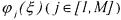may be described by

where

85

Ph. Bogaerts and R. Hanus

• is a kinetic constant (function, if necessary, of any physical influence

different from the component concentrations, e.g., the temperature dependence according to an Arrhenius law);

• the set of indices of the components which activate the reaction j (reactants, catalysts and auto-catalysts);

• the set of indices of all the components appearing in reaction j (or even, if

• the inhibition coefficient of component l in reaction j.

This structure has the advantage to be very general in the sense that the activation and/or the inhibition of the reaction by any component can be taken into account. It is obvious that the kinetic parameters have a physical meaning, namely, the activation and/or inhibition .We will see that this property allows to propose necessary conditions to be satisfied by the reaction scheme. A sufficient condition to guarantee the concentration positiveness is that the activation coefficients are such that

Otherwise, it is necessary to use saturation on the concentration vector

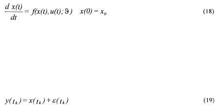
such that the lower bound is equalled to zero. Provided these latter precautions to guarantee the concentration positiveness, the BIBS stability of the system of mass balances (9) using the kinetic model structure (16) is guaranteed if one of the sufficient conditions of Section 2 are satisfied. Finally, the structure (16) is nonlinear w.r.t. the kinetic parameters but may be linearised thanks to a logarithmic transformation. Indeed, the logarithm of both members of eq. (16) leads to

which is linear w.r.t. the parameters

The model structure considered in the sequel is made of the system of mass balances

(5) (based upon the reaction scheme (1)) using the general kinetic model structure (16). The question which arises is the identification of the model parameters (i.e., the pseudo- stoichiometric coefficients and the kinetic coefficients) given a set of experimental data containing measurements of the concentration vector and the corresponding input data (dilution rate, external feed rates).

86

Macroscopic modelling of bioprocesses with a view to engineering applications

4. Parameter identification

4.1. MOTIVATIONS FOR A SYSTEMATIC PROCEDURE

In the same way as for the kinetic model structure, several motivations exist to propose a complete systematic procedure well suited for the problem. Indeed, in several contributions to the mathematical modelling of bioprocesses, it is the model structure that is mainly discussed and neither the parameter identification procedure nor the model validation. Hereafter, several problems often encountered in the literature are summarised.

In some cases, the parameter identification method is not given. For instance, Ramakrishna et al. (1996) just tell that “parameters were estimated from experimental data, literature studies, previous cybernetic modelling efforts, and order-of-magnitude estimations” without any more detail. In other cases, parameter values are just taken from the literature, by using eventually mean values coming from different sources (Martens et al., 1995). Other authors use a trial-and-error method where the model validation criterion is the visual difference between experimental data and simulated values (Goergen et al., 1994; Barford et al., 1992). In most of the studies in the literature, the identification procedure does not take into account the confidence that can be associated with the measurements. For instance, Julien et al. (1998) identify a simulation model for an activated sludge process and compare graphically simulated values and experimental data, these latter being presented with their confidence interval. Although these authors analyse the identification problem much more deeply than in lots of other contributions, they do not use this precious information of the confidence intervals in the cost function of the parameter identification procedure. As an obvious consequence of the last point, the confidence intervals for the identified parameters are rarely provided together with the identified values.

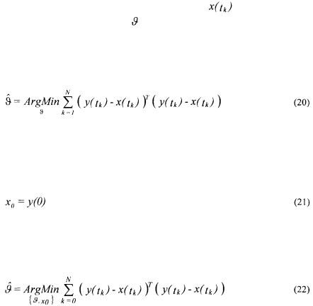
Another important problem in the usual literature is that the initial conditions of a simulation model are generally measured values that are supposed to be infinitely accurate. Let us consider a simulation model given by the differential equation

where

•x(t) is the simulated state vector;

• is the initial state vector;

•u(t) is the input vector;

• is the vector of the model parameters.

For identifying the parameters contained in the vector , sampled measurements are available:

87

white, with Gaussian distribution of zero mean, see paragraph 4.2). In most of the cases

of the literature, the vector is simply identified by minimising a least squares criterion (which is also based on the assumption of a constant standard deviation for the noise):

Given the model (18), the measurements (19) and the above assumptions on the measurement noise, the solution is the one corresponding to the most likely errors . But the measurements at the initial time are treated in a different way from all the other ones as the initial conditions of the simulation model are fixed to

Hence, the solution (20) is meaningful only if the measurement error As there is no reason a priori to satisfy this condition, the only coherent procedure consists in identifying the initial conditions too:

We have proved in (Some et al., 1999) the importance of the identification of the initial conditions in the framework of the estimation of drug stability parameters, namely activation energy and shelf-life of acetylsalicylic acid. Of course, this problem arises in any kind of simulation model.

Another frequent problem is that one measured signal is assumed to be corrupted by noise while the others are supposed to be perfectly known. This assumption is often made (but almost never explicitly) with linear regressions where all the regressors are supposed to be perfectly known. This problem is particularly important in the framework of bioprocess modelling as the pseudo-stoichiometric coefficients are usually identified on the basis of linear regressions (Bastin and Dochain, 1990; Chen and Bastin, 1996; Chotteau, 1995). However, it is unacceptable and completely unrealistic to assume that only one concentration measurement is corrupted by noise while the others are not. The way to overcome this problem is to use a maximum likelihood cost function for the identification instead of a least squares cost function (see paragraph 4.2).

Finally, several model identifications are only validated in “simple validation”. This means that the final test consists in trying to simulate the data that have been used for

88

Macroscopic modelling of bioprocesses with a view to engineering applications

the parameter identification. Of course this is just a necessary condition but not a sufficient one. Indeed, if this test fails then it proves that the structure is not able to reproduce the experimental field. But, the greater the number of parameters to be identified the greater the facility to reproduce the available measurements (together with their noise). If the number of parameters becomes too large, the model is then able to reproduce the specific experiments used for the identification rather than the macroscopic behaviour of the system. The “cross validation” is able to detect this kind of problem. It consists in trying to simulate experimental data which have not been used for the parameter identification, hence verifying the ability of the model to reproduce the system behaviour (or even to extrapolate the system behaviour, which means to reproduce experimental data outside the field delimited by the measurements used for the identification). This test is of crucial importance but is rarely made. Of course, other tests are able to provide valuable information about the model validation, see in

Murray-Smith (1998) or in Walter and Pronzato (1997) for a more detailed discussion.

Generally, any test allowing to verify a posteriori what has been assumed a priori in the identification procedure (especially concerning the noise properties) is really worthy.

In order to tackle the main problems highlighted above, a systematic procedure is proposed in the following paragraph.

4.2. SYSTEMATIC PROCEDURE FOR THE PARAMETER IDENTIFICATION

A three-step procedure has been proposed in Bogaerts (1999). The basics of this methodology are given hereafter.

4.2.1. First step: estimation of the pseudo-stoichiometric coefficients (independently of the kinetic coefficients)

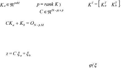
This first step uses the decoupling method proposed in Bastin and Dochain (1990) and in Chen and Bastin (1996). It is always possible to find a full row rank submatrix

(Where is a null matrix). It is then possible to define an auxiliary vector

(24)

89

Ph. Bogaerts and R. Hanus

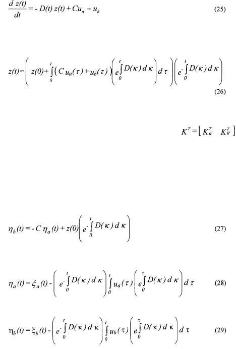
(where corresponds to the partition C can be estimated on the basis of relation (24) where z(t) is obtained by integration of (25):

Considering the particular (but very usual case) where p = rank K = M , a necessary and sufficient condition in order to be able to univocally determine and from relation (23) and the knowledge of C, is that there exists a partition

(with invertible) such that does not contain any unknown coefficient of K (Chen and Bastin, 1996). When this necessary and sufficient condition is satisfied, the model is called C-identifiable. Several solutions are proposed in Bogaerts (1999) in order to estimate the matrix K on the basis of this decoupling method. One of the solutions consists in using a maximum likelihood criterion allowing to take into account all the measurement errors (for each signal and each sample time, including the initial one) and is summarised hereafter.

Let us first inject the solution (26) into the relation (24), which leads to

where

90