

Engineering and Manufacturing for Biotechnology - Marcel Hofman & Philippe Thonart
.pdfMacroscopic modelling of bioprocesses with a view to engineering applications
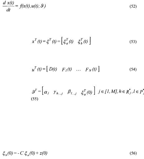
Defining a vector  containing all the unknown parameters of C together with all the initial conditions
  indices of the experiment), its maximum likelihood estimation is given by
where
•
•
•
•
( being the
  sample time of the
  experiment and
  being the
  row of matrix C)
•
•
91
Ph. Bogaerts and R. Hanus
• |
|
• |
|
• |
|
• |
|
• |
|
and |
being white measurement noises, normally distributed, with zero |
mean and covariance matrices  ). All the unknown parameters of
being identified on the basis of (30), an estimation  Finally, the estimations
  of the matrices
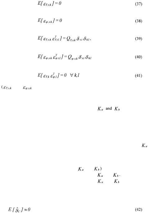
of the matrix C is obtained. are deduced of
equation (23), the existence and uniqueness of the solution being guaranteed by the necessary and sufficient condition of C-identifiability mentioned above.
The signs of the pseudo stoichiometric coefficients in the matrix K are of course imposed by the fact that a given component is consumed in a given reaction (negative coefficient) or is produced in this reaction (positive coefficient). These sign constraints can be verified a posteriori at the end of the (unconstrained) identification procedure proposed above. In some particular cases, the sign constraints on the elements of
and  can be translated in sign constraints on the elements of C (and, consequently, on
  thanks to the relation (23). Then the optimisation problem (30) can be solved under these constraints. Finally, there are some cases (especially when the elements of
C are nonlinear functions of the elements of |
and |
for which it is not possible |
|
anymore to derive the constraints on C from the ones on |
and |
Then the matrix |
|
C may be parameterised in function of the elements of |
and |
and a nonlinear |
|
constrained optimisation problem has to be solved, as shown in Bogaerts (1999).
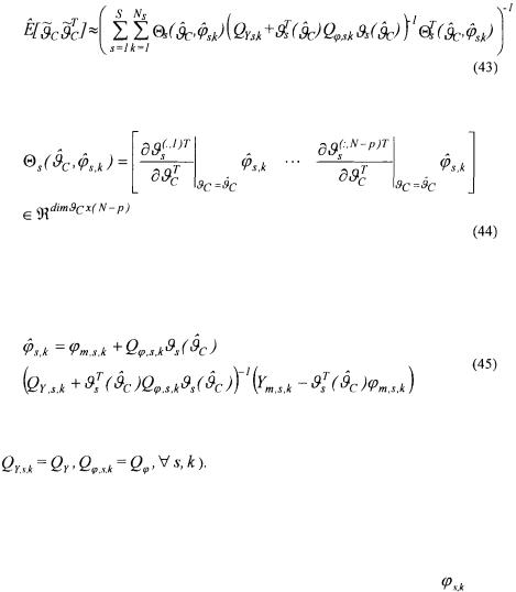
It has also been proved in Bogaerts (1999) that, provided an approximation of first order, the estimate  is unbiased:
92
Macroscopic modelling of bioprocesses with a view to engineering applications
and that an estimation of the covariance matrix of the parameter estimation errors is given by
where
 being the
  column of the matrix
  and
and  being the most likely estimates of the true values
  , given by
Finally, note that the nonlinear optimisation problem (30) only guarantees a unique solution if the measurement noises are time-invariant (which means that
Nevertheless, it is possible to obtain a unique first
initial guess of  in a systematic way. It consists either in considering time invariant matrices for the measurement noise covariance or in reducing the problem to a Markov estimate where the covariance matrix
  is diagonal and the covariance matrix
 Of course this simplification may only serve as unique initial guess
as it relies on the assumption that all the measurements contained in |
are not |
corrupted by noise. Although this assumption is most of the time |
definitely |
unacceptable, this kind of error is often made in the literature. |
|
4.2.2. Second step: first estimation of the kinetic coefficients
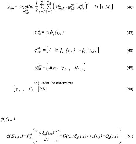
It has been shown that the kinetic model structure (16) can be linearised w.r.t. its parameters thanks to a logarithmic transformation (17). This enables to find a linear least squares estimate of the kinetic coefficients (which necessarily exists, is unique and independent of any initial guess):
93
Ph. Bogaerts and R. Hanus
where
•
•
•
•
Note that the constraints  must be replaced by
  if the concentration positiveness must be guaranteed without using saturations with zero lower bound.
In the very usual case where p = rank K = M, estimates of the reaction rate
can be obtained with the relation
where the estimate of the derivative can, for instance, be computed by the analytical derivation of an interpolation model for the vector  The estimates
  are based on unreliable assumptions on the measurement errors (errors only on
  with
with
constant standard deviation) and on estimates of the signal derivatives. Therefore, these estimates are just considered as a (unique and systematic) initial guess for the last step of the identification.
4.2.3. Third step: final estimation of the kinetic coefficients (and of some initial concentrations
At this step, the identified pseudo-stoichiometric coefficients (determined in the first step) will not be questioned anymore because they were already deduced from a most
94
Macroscopic modelling of bioprocesses with a view to engineering applications
likelihood cost function using reliable assumptions. However, it has been shown that the estimate of the kinetic coefficients computed in the second step is based on unreliable assumptions and may only serve as initial guess of a final nonlinear identification that is the aim of this third step. Together with these kinetic coefficients, (part of) the initial concentrations of the simulation model will also be identified, in agreement with the discussion on the initial conditions of a simulation model given in the previous paragraph.
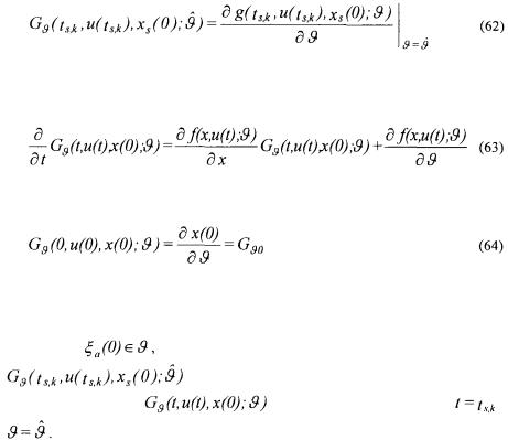
The simulation model {(5),(16)} consists of a nonlinear differential system of the form
where
•
is the state vector containing the concentrations of the components involved in the reaction scheme (1);
•
is the input vector containing the dilution rate and the external feed rates;
•
is the vector of the parameters to be identified (kinetic coefficients and initial concentrations);
• |
f is the model structure corresponding to relations {(5),(16)}. |
Note that the vector  only contains the initial concentrations
  , the other ones
  being deduced from relation (27) which reduces, at time t = 0 , to
where C and z(0) have been identified in the first step of the identification procedure. On the basis of this property, it is also possible to reduce (especially in the batch case
95

Ph. Bogaerts and R. Hanus
where  ) the system of N differential equations (52) in a system of p (rank
of matrix K) differential equations, relative to |
the |
part of the |
state |
vector, |
and |
N - p algebraic equations deduced from (27), |
relative |
to the |
part |
of the |
state |
vector. Details are given in Bogaerts (1999). |
|
|
|
|
|
Let |
|
|
|
|
|
be the solution (generally obtained by numerical solving) of the differential system (52) starting from the initial concentrations  On the basis of sampled measurements
being the  sample time of the
  experiment) corrupted by white measurement
noise |
normally distributed with zero mean and covariance matrix |
the |
maximum likelihood estimate of  can then be deduced from a nonlinear Markov estimator
under the constraints
The initial guess of  consists, on the one hand, of the first estimate of the kinetic parameters deduced from the second step of the procedure and, on the other hand, of the
measurements of |
at the initial time. |
The covariance matrix of the parameter estimation errors can also be estimated in this last step (Bogaerts, 1999):
96
Macroscopic modelling of bioprocesses with a view to engineering applications
where
This Jacobian is obtained by solving (together with the simulation model (52) ) the sensitivity equations
with the initial condition
where  is a matrix whose elements are all equalled to zero except the ones giving the partial derivative of the elements of
  w.r.t. the corresponding
elements of |
these partial derivatives being equalled to |
1. The |
Jacobian |
|
involved in relation (61) is thus obtained by evaluating |
||
the numerical solution |
of the system {(52),(63)} |
for |
and |
At the end of this third step, all the parameters have been identified: the pseudostoichiometric coefficients in the first step (30) and the kinetic coefficients in the third step (59). Hence, the model is completely determined but has of course to be validated (cross validation, study of the correlation matrix of the parametric errors, etc., see in (Bogaerts, 1999) ). Note that it is also possible to build confidence intervals for simulation trajectories obtained with the model identified with the above mentioned procedure (Bogaerts, 1999). This allows to quantify the uncertainty in the simulation results coming from the uncertainty on the identified parameters. Finally, the following paragraph provides necessary conditions for the validation of the reaction scheme (1) on the basis of the identified parameters.
4.3. NECESSARY CONDITIONS FOR REACTION SCHEME VALIDATION
The results provided by the three-step identification procedure can be used to determine necessary conditions for the reaction scheme validation. A first one is a “good” level of validation of the linear relations (27) which allow to identify the pseudo-stoichiometric coefficients. Of course this “good” level can be quantified in several ways (e.g., on the
97
Ph. Bogaerts and R. Hanus
basis of linear regression coefficients). If the validation tests fail then it is obvious that the reaction scheme can not be used to reproduce the experiments. However, a good validation is absolutely not a sufficient condition of reaction scheme validation because several reaction schemes may lead to the same linear relations (27).
Another valuable information is provided by the eventual activation of the sign
constraints on the activation coefficients |
coupled with the sign of |
the corresponding pseudo-stoichiometric coefficient |
Several cases may arise: |
•If  and
and  (non activated constraint), then the component
  is
is
consumed by the reaction and activates this latter. Hence, it consists of a simple reactant.
• However, if  and
and  (activated constraint), then the component
is consumed by the  reaction but does not activate this latter. This is not very meaningful and could lead to negative concentrations if these latter are not artificially saturated with a zero lower bound. Even if saturations are used, this case is not really acceptable from a physical point of view and highlights probably the narrow limits of the validation field. Consequently, it is preferable to modify such a reaction by taking this reactant away.
•If  and
and  (non activated constraint), then the component
  is
is
produced by the  reaction and activates this latter. Hence, it consists of an autocatalyst for the considered reaction.
•However, if  and
and  (activated constraint), then the component
  is produced by the
  reaction but does not activate this latter. This means that this
component is a simple product and is not an autocatalyst. If this component corresponds to the biomass, then the considered reaction is out of sense because it should allow the simulation of spontaneous growth of living microorganisms
(without any living cell present at the initial time of the experiment).
•If  and
and  (non activated constraint), then the component
  is
is
neither consumed nor produced by the reaction but activates this latter. Hence, it consists of a catalyst for the considered reaction.
•However, if  and
and  (activated constraint), then the component
  is neither consumed nor produced by the
  reaction and does not activate this latter. It does not take place in the considered reaction and may be taken away from
it.
In summary, the following propositions are necessary conditions for the reaction scheme validation, which can be verified on the basis of the parameter identification results:
•it is necessary to reach a “good” level of validation of the linear relations (27) which allow to identify the pseudo-stoichiometric coefficients;
•a component which is supposed to be a reactant, a catalyst or an autocatalyst in a given reaction must be characterised by a strictly positive activation coefficient in this reaction.
98
Macroscopic modelling of bioprocesses with a view to engineering applications
5. Application on simulated bacteria cultures
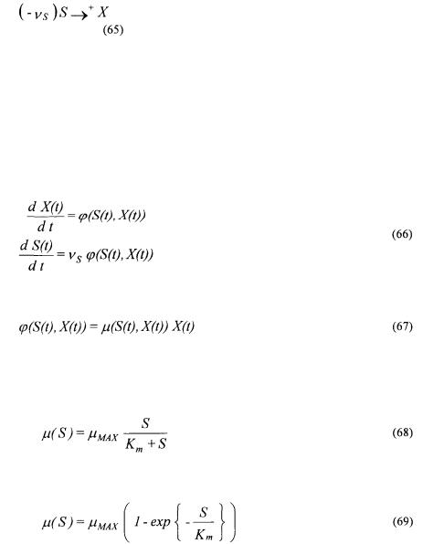
In order to test the flexibility of the new general kinetic model structure presented in Section 3, a simulator of batch bacterial cultures is built with the software MATLAB 5.2. The reaction scheme corresponds to the growth reaction
where
•S is the substrate;
•X is the biomass;
• is a (negative) pseudo-stoichiometric coefficient;
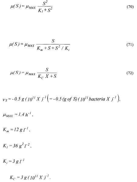
• denotes an autocatalytic reaction (X being the autocatalyst). The mass balances of X and S are then given by
where the growth rate
is such that the specific growth rate  is described by one of the following well known model structures.
• |
Monod (limitation by S): |
• |
Tessier (limitation by S): |
99
Ph. Bogaerts and R. Hanus
• |
Ming (limitation by S): |
•Haldane (limitation and inhibition by S):
• Contois (limitation by S and inhibition by X ):
The following numerical values are used:
and
Note that these values of  and
and  were used by Holmberg (1983) in order to
model a culture of bacteria B. thuringiensis in a study on the identifiability problems with the Monod law.
The simulator {(66),(67)} (together with one of the laws {(68),...,(72)} ) has been used for generating, in each of the five cases of specific growth rate, two experiments
100