Handbook_of_statistical_analysis_using_SAS

Fitted Distribution for Hardness

Parameters for Normal Distribution

©2002 CRC Press LLC

Quantiles for Normal Distribution

Display 2.3

The quantiles provide information about the tails of the distribution as well as including the five number summaries for each variable. These consist of the minimum, lower quartile, median, upper quartile, and maximum values of the variables. The box plots that can be constructed from these summaries are often very useful in comparing distributions and identifying outliers. Examples are given in subsequent chapters.

The listing of extreme values can be useful for identifying outliers, especially when used with an id statement. The following section, entitled “Fitted Distribution for Hardness,” gives details of the distribution fitted to the histogram. Because a normal distribution is fitted in this instance, it largely duplicates the output generated by the normal option on the proc statement.

The numerical information in Display 2.2 and the plots in Displays 2.4 and 2.5 all indicate that mortality is symmetrically, approximately normally, distributed. The formal tests of normality all result in non-significant values of the test statistic. The results in Display 2.3 and the plots in Displays 2.6 and 2.7, however, strongly suggest that calcium concentration (hardness) has a skew distribution with each of the tests for normality having associated P-values that are very small.

©2002 CRC Press LLC

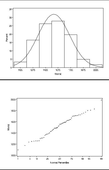
Display 2.4

Display 2.5

©2002 CRC Press LLC

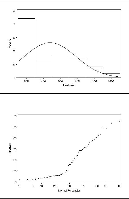
Display 2.6

Display 2.7

©2002 CRC Press LLC

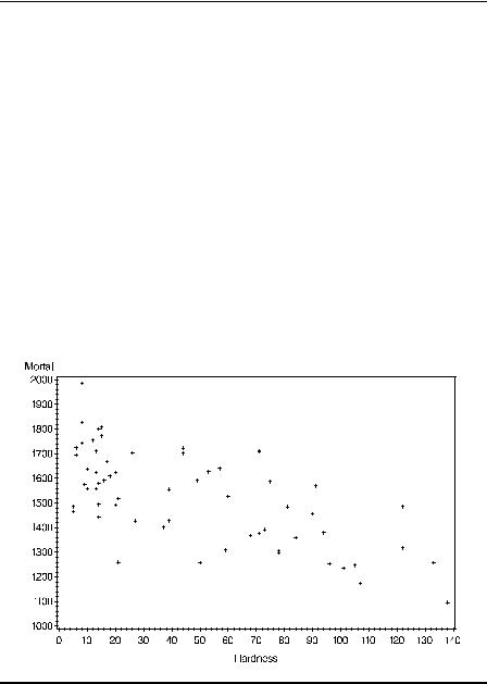
The first step in examining the relationship between mortality and water hardness is to look at the scatterplot of the two variables. This can be found using proc gplot with the following instructions:

proc gplot;

plot mortal*hardness; run;

The resulting graph is shown in Display 2.8. The plot shows a clear negative association between the two variables, with high levels of calcium concentration tending to occur with low mortality values and vice versa. The correlation between the two variables is easily found using proc corr, with the following instructions:

proc corr data=water pearson spearman; var mortal hardness;

run;

Display 2.8

The pearson and spearman options in the proc corr statement request that both types of correlation coefficient be calculated. The default, if neither option is used, is the Pearson coefficient.

©2002 CRC Press LLC

The results from these instructions are shown in Display 2.9. The correlation is estimated to be –0.655 using the Pearson coefficient and –0.632 using Spearman’s coefficient. In both cases, the test that the population correlation is zero has an associated P-value of 0.0001. There is clearly strong evidence for a non-zero correlation between the two variables.

The CORR Procedure

2 Variables: Mortal Hardness

Pearson Correlation Coefficients, N = 61

Prob > |r| under H0: Rho=0

Spearman Correlation Coefficients, N = 61

Prob > |r| under H0: Rho=0

Display 2.9

One of the questions of interest about these data is whether or not there is a geographical factor in the relationship between mortality and water hardness, in particular whether this relationship differs between the

©2002 CRC Press LLC

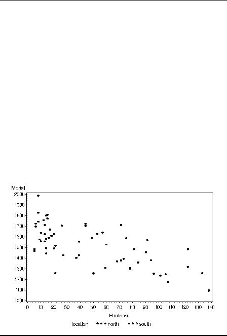
towns in the North and those in the South. To examine this question, a useful first step is to replot the scatter diagram in Display 2.8 with northern and southern towns identified with different symbols. The necessary instructions are

symbol1 value=dot; symbol2 value=circle; proc gplot;

plot mortal*hardness = location; run;

The plot statement of the general form plot y * x = z will result in a scatter plot of y by x with a different symbol for each value of z. In this case, location has only two values and the first two plotting symbols used by SAS are 'x'and '+'. The symbol statements change the plotting symbols to give more impact to the scattergram.

The resulting plot is shown in Display 2.10. There appears to be no obvious difference in the form of the relationship between mortality and hardness for the two groups of towns.

Display 2.10

©2002 CRC Press LLC

Separate correlations for northern and southern towns can be produced using proc corr with a by statement as follows:

proc sort;

by location;

proc corr data=water pearson spearman; var mortal hardness;

by location; run;

The by statement has the effect of producing separate analyses for each subgroup of the data defined by the specified variable, location in this case. However, the data set must first be sorted by that variable.

The results from this series of instructions are shown in Display 2.11. The main items of interest in this display are the correlation coefficients and the results of the tests that the population correlations are zero. The Pearson correlation for towns in the North is –0.369, and for those in the South it is –0.602. Both values are significant beyond the 5% level. The Pearson and Spearman coefficients take very similar values for this example.

Pearson Correlation Coefficients, N = 35

Prob > |r| under H0: Rho=0

©2002 CRC Press LLC

Spearman Correlation Coefficients, N = 35

Prob > |r| under H0: Rho=0

Display 2.11

©2002 CRC Press LLC

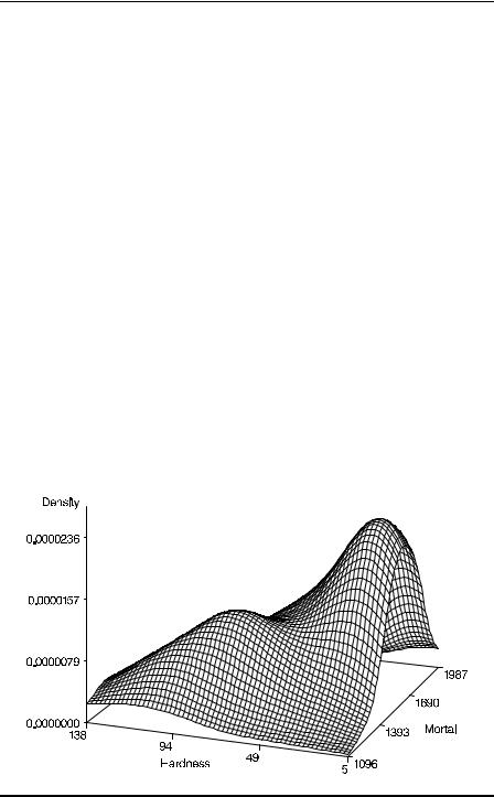
Examination of scatterplots often centres on assessing density patterns such as clusters, gaps, or outliers. However, humans are not particularly good at visually examining point density and some type of density estimate added to the scatterplot is frequently very helpful. Here, plotting a bivariate density estimate for mortality and hardness is useful for gaining more insight into the structure of the data. (Details on how to calculate bivariate densities are given in Silverman [1986].) The following code produces and plots the bivariate density estimate of the two variables:

proc kde data=water out=bivest; var mortal hardness;

proc g3d data=bivest;

plot hardness*mortal=density; run;

The KDE procedure (proc kde) produces estimates of a univariate or bivariate probability density function using kernel density estimation (see Silverman [1986]). If a single variable is specified in the var statement, a univariate density is estimated and a bivariate density if two are specified. The out=bivest option directs the density estimates to a SAS data set. These can then be plotted with the three-dimensional plotting procedure proc g3d. The resulting plot is shown in Display 2.12. The two clear modes in the diagram correspond, at least approximately, to northern and southern towns.

Display 2.12

©2002 CRC Press LLC