Handbook_of_statistical_analysis_using_SAS

NOTE: The X'X matrix has been found to be singular, and a generalized inverse was used to solve the normal equations. Terms whose estimates are followed by the letter 'B' are not uniquely estimable.

Display 10.10

Exercises

10.1The graph in Display 10.3 indicates the phenomenon known as “tracking,” the tendency of women with higher depression scores at the beginning of the trial to be those with the higher scores at the end. This phenomenon becomes more visible if standardized scores are plotted [i.e., (depression scores – visit mean)/visit S.D.]. Calculate and plot these scores, differentiating on the plot the women in the two treatment groups.

10.2Apply the response feature approach described in the text, but now using the slope of each woman’s depression score on time as the summary measure.

©2002 CRC Press LLC

Chapter 11

Longitudinal Data II: The

Treatment of Alzheimer’s

Disease

11.1Description of Data

The data used in this chapter are shown in Display 11.1. They arise from an investigation of the use of lecithin, a precursor of choline, in the treatment of Alzheimer’s disease. Traditionally, it has been assumed that this condition involves an inevitable and progressive deterioration in all aspects of intellect, self-care, and personality. Recent work suggests that the disease involves pathological changes in the central cholinergic system, which might be possible to remedy by long-term dietary enrichment with lecithin. In particular, the treatment might slow down or perhaps even halt the memory impairment associated with the condition. Patients suffering from Alzheimer’s disease were randomly allocated to receive either lecithin or placebo for a 6-month period. A cognitive test score giving the number of words recalled from a previously given standard list was recorded monthly for 5 months.

The main question of interest here is whether the lecithin treatment has had any effect.

©2002 CRC Press LLC

©2002 CRC Press LLC

1 = Placebo, 2 = Lecithin

Display 11.1

11.2Random Effects Models

Chapter 10 considered some suitable graphical methods for longitudinal data, and a relatively straightforward inferential procedure. This chapter considers a more formal modelling approach that involves the use of random effects models. In particular, we consider two such models: one that allows the participants to have different intercepts of cognitive score on time, and the other that also allows the possibility of the participants having different slopes for the regression of cognitive score on time.

Assuming that yijk represents the cognitive score for subject k on visit j in group i, the random intercepts model is

where β 0, β 1, and β 2 are respectively the intercept and regression coefficients for Visit and Group (where Visit takes the values 1, 2, 3, 4, and 5, and Group the values 1 for placebo and 2 for lecithin); ak are random effects that model the shift in intercept for each subject, which because there is a fixed change for visit, are preserved for all values of visit; and the ijk are residual or error terms. The ak are assumed to have a normal distribution with mean zero and variance σ a2 . The ijk are assumed to have a normal distribution with mean zero and variance σ 2. Such a model implies a compound symmetry covariance pattern for the five repeated measures (see Everitt [2001] for details).

The model allowing for both random intercept and random slope can be written as:

©2002 CRC Press LLC

Now a further random effect has been added to the model compared to Eq. (11.1). The terms bk are assumed to be normally distributed with mean zero and variance σ b2 . In addition, the possibility that the random effects are not independent is allowed for by introducing a covariance term for

them, σ ab.

The model in Eq. (11.2) can be conveniently written in matrix notation

The model implies the following covariance matrix for the repeated measures:

where

©2002 CRC Press LLC

Details of how to fit such models are given in Pinheiro and Bates (2000).

11.3Analysis Using SAS

We assume that the data shown in Display 11.1 are in an ASCII file, alzheim.dat, in the current directory. The data step below reads the data and creates a SAS data set alzheim, with one case per measurement. The grouping variable and five monthly scores for each subject are read in together, and then split into separate o bservations using the array, iterative do loop, and output statement. This technique is described in more detail in Chapter 5. The automatic SAS variable _n_ is used to form a subject identifier. With 47 subjects and 5 visits each, the resulting data set contains 235 observations.

data alzheim;

infile 'alzheim.dat';

input group score1-score5; array sc {5} score1-score5; idno=_n_;

do visit=1 to 5; score=sc{visit}; output;

end;

run;

We begin with some plots of the data. First, the data are sorted by group so that the by statement can be used to produce separate plots for each group.

proc sort data=alzheim; by group;

run;

symbol1 i=join v=none r=25; proc gplot data=alzheim;

plot score*visit=idno / nolegend;

©2002 CRC Press LLC

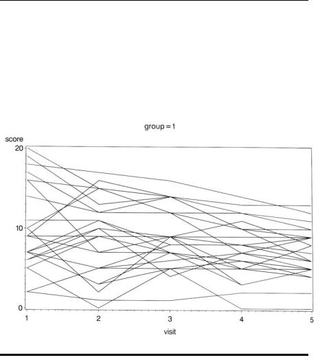
by group; run;

To plot the scores in the form of a line for each subject, we use plot score*visit=idno. There are 25 subjects in the first group and 22 in the second. The plots will be produced separately by group, so the symbol definition needs to be repeated 25 times and the r=25 options does this. The plots are shown in Displays 11.2 and 11.3.

Display 11.2

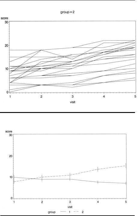
Next we plot mean scores with their standard errors for each group on the same plot. (See Chapter 10 for an explanation of the following SAS statements.) The plot is shown in Display 11.4.

goptions reset=symbol; symbol1 i=std1mj v=none l=1; symbol2 i=std1mj v=none l=3; proc gplot data=alzheim;

plot score*visit=group; run;

©2002 CRC Press LLC

Display 11.3

Display 11.4

©2002 CRC Press LLC

The random intercepts model specified in Eq. (11.1) can be fitted using proc mixed, as follows:

proc mixed data=alzheim method=ml; class group idno;

model score=group visit /s outpred=mixout; random int /subject=idno;

run;

The proc statement specifies maximum likelihood estimation (method=ml) rather than the default, restricted maximum likelihood (method=reml), as this enables nested models to be compared (see Pinheiro and Bates, 2000). The class statement declares the variable group as a factor, but also the subject identifier idno. The model statement specifies the regression equation in terms of the fixed effects. The specification of effects is the same as for proc glm described in Chapter 6. The s (solution) option requests parameter estimates for the fixed effects and the outpred option specifies that the predicted values are to be saved in a data set mixout. This will also contain all the variables from the input data set alzheim.

The random statement specifies which random effects are to be included in the model. For the random intercepts model, int (or intercept) is specified. The subject= option names the variable that identifies the subjects in the data set. If the subject identifier, idno in this case, is not declared in the class statement, the data set should be sorted into subject identifier order.

The results are shown in Display 11.5. We see that the parameters σ a2 and σ 2 are estimated to be 15.1284 and 8.2462, respectively (see “Covariance Parameter Estimates”). The tests for the fixed effects in the model indicate that both group and visit are significant. The parameter estimate for group indicates that group 1 (the placebo group) has a lower average cognitive score. The estimated treatment effect is –3.06, with a 95% confidence interval of –3.06 ± 1.96 × 1.197, that is, (–5.41, –0.71). The goodness- of-fit statistics given in Display 11.5 can be used to compare models (see later). In particular the AIC (Akaike’s Information Criterion) tries to take into account both the statistical goodness-of-fit and the number of parameters needed to achieve this fit by imposing a penalty for increasing the number of parameters (for more details, see Krzanowski and Marriott [1995]).

Line plots of the predicted values for each group can be obtained as follows:

symbol1 i=join v=none l=1 r=30; proc gplot data=mixout;

plot pred*visit=idno / nolegend;

©2002 CRC Press LLC

by group; run;

The plots are shown in Displays 11.6 and 11.7.

©2002 CRC Press LLC