Handbook_of_statistical_analysis_using_SAS

Display 14.5

Display 14.6

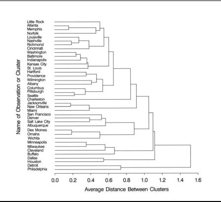
We see in Display 14.5 that complete linkage clustering begins with the same initial “fusions” of pairs of cities as single linkage, but eventually

©2002 CRC Press LLC

begins to join different sets of observations. The corresponding dendrogram in Display 14.6 shows a little more structure, although the number of groups is difficult to assess both from the dendrogram and using the CCC criterion.

The CLUSTER Procedure

Average Linkage Cluster Analysis

Eigenvalues of the Correlation Matrix

The data have been standardized to mean 0 and variance 1 Root-Mean-Square Total-Sample Standard Deviation = 1

Root-Mean-Square Distance Between Observations = 3.464102

©2002 CRC Press LLC

Display 14.7

The average linkage results in Display 14.7 are more similar to those of complete linkage than single linkage; and again, the dendrogram (Display 14.8) suggests more evidence of structure, without making the optimal number of groups obvious.

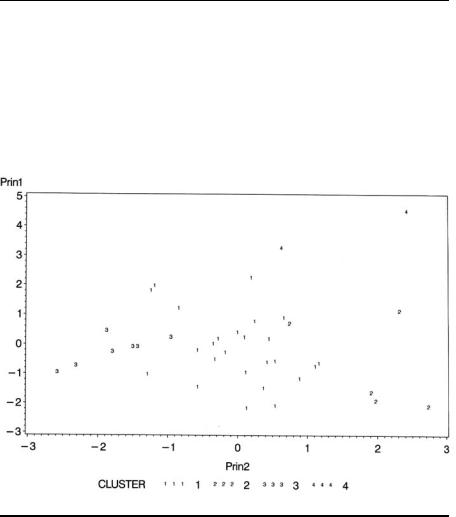
It is often useful to display the solutions given by a clustering technique by plotting the data in the space of the first two or three principal components and labeling the points by the cluster to which they have been assigned. The number of groups that we should use for these data is not clear from the previous analyses; but to illustrate, we will show the four-group solution obtained from complete linkage.

proc tree data=complete out=clusters n=4 noprint; copy city so2 temperature--rainydays;

run;

As well as producing a dendrogram, proc tree can also be used to create a data set containing a variable, cluster, that indicates to which of a specified number of clusters each observation belongs. The number of clusters is specified with the n= option. The copy statement transfers the named variables to this data set.

The mean vectors of the four groups are also useful in interpretation. These are obtained as follows and the output shown in Display 14.9.

©2002 CRC Press LLC

Display 14.8

proc sort data=clusters; by cluster;

©2002 CRC Press LLC

Display 14.9

A plot of the first two principal components showing cluster membership can be produced as follows. The result is shown in Display 14.10.

proc princomp data=clusters n=2 out=pcout noprint; var temperature--rainydays;

©2002 CRC Press LLC

proc gplot data=pcout; symbol1 v='1'; symbol2 v='2'; symbol3 v='3'; symbol4 v='4';

plot prin1*prin2=cluster; run;

Display 14.10

We see that this solution contains three clusters containing only a few observations each, and is perhaps not ideal. Nevertheless, we continue to use it and look at differences between the derived clusters in terms of differences in air pollution as measured by their average SO2 values. Box plots of SO2 values for each of the four clusters can be found as follows:

proc boxplot data=clusters; plot so2*cluster;

run;

The plot is shown in Display 14.11.

©2002 CRC Press LLC

Display 14.11

More formally, we might test for a cluster difference in SO2 values using a one-way analysis of variance. Here we shall use proc glm for the analysis. The output is shown in Display 14.12.

proc glm data=clusters; class cluster;

model so2=cluster; run;

The GLM Procedure

Class Level Information

Number of observations 39

©2002 CRC Press LLC

Display 14.12

The analysis suggests that there is a significant difference in SO2 levels in the four clusters.

This probable difference might be investigated in more detail using a suitable multiple comparison procedure (see Exercise 14.4).

Exercises

14.1Explore some of the other clustering procedures available in SAS; for example, proc modeclus, on the air pollution data.

14.2Repeat the cluster analysis described in this chapter, but now including the data on Chicago and Phoenix.

14.3In the cluster analysis described in the text, the data were standardized prior to clustering to unit standard deviation for each variable. Repeat the analysis when the data are standardized by the range instead.

©2002 CRC Press LLC

14.4Use a multiple comparison procedure to investigate which particular clusters in the complete linkage solution differ in air pollution level.

©2002 CRC Press LLC

Chapter 15

Discriminant Function

Analysis: Classifying

Tibetan Skulls

15.1Description of Data

In the 1920s, Colonel Waddell collected 32 skulls in the southwestern and eastern districts of Tibet. The collection comprised skulls of two types:

Type A: 17 skulls from graves in Sikkim and neighbouring areas of Tibet

Type B: 15 skulls picked up on a battlefield in the Lhausa district and believed to be those of native soldiers from the eastern province of Kharis

It was postulated that Tibetans from Kharis might be survivors of a particular fundamental human type, unrelated to the Mongolian and Indian types that surrounded them.

A number of measurements were made on each skull and Display 15.1 shows five of these for each of the 32 skulls collected by Colonel Waddell. (The data are given in Table 144 of SDS.) Of interest here is whether the two types of skull can be accurately classified from the five measurements

©2002 CRC Press LLC