Handbook_of_statistical_analysis_using_SAS

For an interaction effect to be allowed in the model, all the lower-order interactions and main effects that it implies must also be included.

The results are given in Display 8.7. We see that both the fibrinogen × γ -globulin interaction effect and the γ -globulin main effect are eliminated from the initial model. It appears that only fibrinogen level is predictive of ESR level.

The LOGISTIC Procedure

Model Information

Backward Elimination Procedure

Step 0. The following effects were entered:

Intercept fibrinogen gamma fibrinogen*gamma

Model Convergence Status

Convergence criterion (GCONV=1E-8) satisfied.

Model Fit Statistics

©2002 CRC Press LLC

Testing Global Null Hypothesis: BETA=0

Step 1. Effect fibrinogen*gamma is removed:

Model Convergence Status

Convergence criterion (GCONV=1E-8) satisfied.

The LOGISTIC Procedure

Model Fit Statistics

Residual Chi-Square Test

Step 2. Effect gamma is removed:

Model Convergence Status

Convergence criterion (GCONV=1E-8) satisfied.

©2002 CRC Press LLC

Model Fit Statistics

Testing Global Null Hypothesis: BETA=0·

Residual Chi-Square Test

NOTE: No (additional) effects met the 0.05 significance level for removal from the model.

©2002 CRC Press LLC

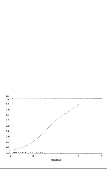
Display 8.7

It is useful to look at a graphical display of the final model selected and the following code produces a plot of predicted values from the fibrinogen-only logistic model along with the observed values of ESR (remember that these can only take the values of 0 or 1). The plot is shown in Display 8.8.

Display 8.8

©2002 CRC Press LLC

proc logistic data=plasma desc; model esr=fibrinogen;

output out=lout p=lpred;

proc sort data=lout; by fibrinogen;

symbol1 i=none v=circle; symbol2 i=join v=none; proc gplot data=lout;

plot (esr lpred)*fibrinogen /overlay ; run;

Clearly, an increase in fibrinogen level is associated with an increase in the probability of the individual being categorised as unhealthy.

8.3.3 Danish Do-It-Yourself

Assuming that the data shown in Display 8.3 are in a file 'diy.dat'in the current directory and the values are separated by tabs, the following data step can be used to create a SAS data set for analysis. As in previous examples, the values of the grouping variables can be determined from the row and column positions in the data. An additional feature of this data set is that each cell of the design contains two data values: counts of those who answered “yes” and “no” to the question about work in the home. Each observation in the data set needs both of these values so that the events/trials syntax can be used in proc logistic. To do this, two rows of data are input at the same time: six counts of “yes” responses and the corresponding “no” responses.

data diy;

infile 'diy.dat' expandtabs; input y1-y6 / n1-n6;

length work $9.; work='Skilled';

if _n_ > 2 then work='Unskilled'; if _n_ > 4 then work='Office';

if _n_ in(1,3,5) then tenure='rent'; else tenure='own';

array yall {6} y1-y6;

©2002 CRC Press LLC

array nall {6} n1-n6; do i=1 to 6;

if i>3 then type='house'; else type='flat';

agegrp=1;

if i in(2,5) then agegrp=2; if i in(3,6) then agegrp=3;

yes=yall{i};

no=nall{i};

total=yes+no;

prdiy=yes/total;

output;

end;

drop i y1--n6; run;

The expandtabs option in the infilestatement allows list input to be used. The input statement reads two lines of data from the file. Six data values are read from the first line into variables y1 to y6. The slash that follows tells SAS to go to the next line and six values from there are read into variables n1 to n6.

There are 12 lines of data in the file; but because each pass through the data step is reading a pair of lines, the automatic variable _n_ will range from 1 to 6. The appropriate values of the work and tenure variables can then be assigned accordingly. Both are character variables and the length statement specifies that work is nine characters. Without this, its length would be determined from its first occurrence in the data step. This would be the statement work='skilled’; and a length of seven characters would be assigned, insufficient for the value 'unskilled'.

The variables containing the yes and no responses are declared as arrays and processed in parallel inside a do loop. The values of age group and accommodation type are determined from the index of the do loop (i.e., from the column in the data). Counts of yes and corresponding no responses are assigned to the variables yes and no, their sum assigned to total, and the observed probability of a yes to prdiy. The output statement within the do loop writes six observations to the data set. (See Chapter 5 for a more complete explanation.)

As usual with a complicated data step such as this, it is wise to check the results; for example, with proc print.

A useful starting point in examining these data is a tabulation of the observed probabilities using proc tabulate:

©2002 CRC Press LLC

proc tabulate data=diy order=data f=6.2; class work tenure type agegrp;

var prdiy;

table work*tenure all, (type*agegrp all)*prdiy*mean;

run;

Basic use of proc tabulate was described in Chapter 5. In this example, the f= option specifies a format for the cell entries of the table, namely six columns with two decimal places. It also illustrates the use of the keyword all for producing totals. The result is shown in Display 8.9. We see that there are considerable differences in the observed probabilities, suggesting that some, at least, of the explanatory variables may have an effect.

Display 8.9

We continue our analysis of the data with a backwards elimination logistic regression for the main effects of the four explanatory variables only.

proc logistic data=diy;

class work tenure type agegrp /param=ref ref=first;

model yes/total=work tenure type agegrp / selection=back ward;

run;

©2002 CRC Press LLC

All the predictors are declared as classfication variables, or factors, on the class statement. The param option specifies reference coding (more commonly referred to as dummy variable coding), with the ref option setting the first category to be the reference category. The output is shown in Display 8.10.

The LOGISTIC Procedure

Model Information

Backward Elimination Procedure

Class Level Information

©2002 CRC Press LLC

Step 0. The following effects were entered:

Intercept work tenure type agegrp

Model Convergence Status

Convergence criterion (GCONV=1E-8) satisfied.

Model Fit Statistics

The LOGISTIC Procedure

Testing Global Null Hypothesis: BETA=0

Step 1. Effect type is removed:

Model Convergence Status

Convergence criterion (GCONV=1E-8) satisfied.

Model Fit Statistics

©2002 CRC Press LLC

Testing Global Null Hypothesis: BETA=0

0.0003 1 0.9865

NOTE: No (additional) effects met the 0.05 significance level for removal from the model.

Summary of Backward Elimination

©2002 CRC Press LLC