Handbook_of_statistical_analysis_using_SAS

The output statement specifies that the predicted values and standardized Pearson (Chi) residuals are to be saved in the variables pr_days and resid, respectively, in the data set genout.

The new results are shown in Display 9.4. Allowing for overdispersion has had no effect on the regression coefficients, but a large effect on the P-values and confidence intervals so that sex and type are no longer significant. Interpretation of the significant effect of, for example, origin is made in terms of the logs of the predicted mean counts. Here, the estimated coefficient for origin 0.4951 indicates that the log of the predicted mean number of days absent from school for Aboriginal children is 0.4951 higher than for white children, conditional on the other variables. Exponentiating the coefficient yield count ratios, that is, 1.64 with corresponding 95% confidence interval (1.27, 2.12). Aboriginal children have between about one and a quarter to twice as many days absent as white children.

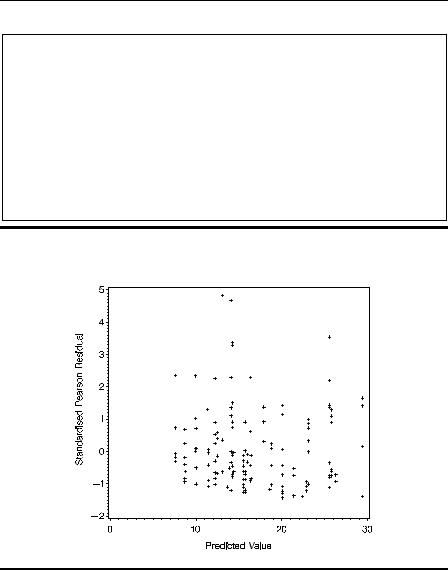
The standardized residuals can be plotted against the predicted values using proc gplot.

proc gplot data=genout; plot resid*pr_days;

run;

The result is shown in Display 9.5. This plot does not appear to give any cause for concern.

The GENMOD Procedure

Model Information

Class Level Information

©2002 CRC Press LLC

Criteria For Assessing Goodness Of Fit

Algorithm converged.

Analysis Of Parameter Estimates

NOTE: The scale parameter was held fixed.

LR Statistics For Type 1 Analysis

©2002 CRC Press LLC

The GENMOD Procedure

LR Statistics For Type 3 Analysis

Display 9.4

Display 9.5

Exercises

9.1Test the significance of the interaction between class and race when using a Poisson model for the Australian school children data.

©2002 CRC Press LLC

9.2Dichotomise days absent from school by classifying 14 days or more as frequently absent. Analyse this new response variable using both the logistic and probit link and the binomial family.

©2002 CRC Press LLC

Chapter 10

Longitudinal Data I: The

Treatment of Postnatal

Depression

10.1Description of Data

The data set to be analysed in this chapter originates from a clinical trial of the use of oestrogen patches in the treatment of postnatal depression. Full details of the study are given in Gregoire et al. (1998). In total, 61 women with major depression, which began within 3 months of childbirth and persisted for up to 18 months postnatally, were allocated randomly to the active treatment or a placebo (a dummy patch); 34 received the former and the remaining 27 received the latter. The women were assessed twice pretreatment and then monthly for 6 months after treatment on the Edinburgh postnatal depression scale (EPDS), higher values of which indicate increasingly severe depression. The data are shown in Display 10.1. A value of –9 in this table indicates that the corresponding observation was not made for some reason.

©2002 CRC Press LLC

©2002 CRC Press LLC

0 = Placebo, 1 = Active

Display 10. 1

10.2The Analyses of Longitudinal Data

The data in Display 10.1 consist of repeated observations over time on each of the 61 patients; they are a particular form of repeated measures data (see Chapter 7), with time as the single within-subjects factor. The analysis of variance methods described in Chapter 7 could be, and frequently are, applied to such data; but in the case of longitudinal data, the sphericity assumption is very unlikely to be plausible — observations closer together in time are very likely more highly correlated than those taken further apart. Consequently, other methods are generally more useful for this type of data. This chapter considers a number of relatively simple approaches, including:

Graphical displays

Summary measure or response feature analysis

Chapter 11 discusses more formal modelling techniques that can be used to analyse longitudinal data.

10.3Analysis Using SAS

Data sets for longitudinal and repeated measures data can be structured in two ways. In the first form, there is one observation (or case) per

©2002 CRC Press LLC

subject and the repeated measurements are held in separate variables. Alternatively, there may be separate observations for each measurement, with variables indicating which subject and occasion it belongs to. When analysing longitudinal data, both formats may be needed. This is typically achieved by reading the raw data into a data set in one format and then using a second data step to reformat it. In the example below, both types of data set are created in the one data step.

We assume that the data are in an ASCII file 'channi.dat'in the current directory and that the data values are separated by spaces.

data pndep(keep=idno group x1-x8) pndep2(keep=idno group time dep);

infile 'channi.dat'; input group x1-x8; idno=_n_;

array xarr {8} x1-x8; do i=1 to 8;

if xarr{i}=-9 then xarr{i}=.; time=i;

dep=xarr{i}; output pndep2;

end;

output pndep; run;

The data statement contains the names of two data sets, pndep and pndep2, indicating that two data sets are to be created. For each, the keep= option in parentheses specifies which variables are to be retained in each. The input statement reads the group information and the eight depression scores. The raw data comprise 61 such lines, so the automatic SAS variable _n_ will increment from 1 to 61 accordingly. The variable idno is assigned its value to use as a case identifier because _n_ is not stored in the data set itself.

The eight depression scores are declared an array and a do loop processes them individually. The value –9 in the data indicates a missing value and these are reassigned to the SAS missing value by the if-then statement. The variable time records the measurement occasion as 1 to 8 and dep contains the depression score for that occasion. The output statement writes an observation to the data set pndep2. From the data statement we can see that this data set will contain the subject identifier, idno, plus group, time, and dep. Because this output statement is within

©2002 CRC Press LLC

the do loop, it will be executed for each iteration of the do loop (i.e., eight times).

The second output statement writes an observation to the pndep data set. This data set contains idno, group, and the eight depression scores in the variables x1 to x8.

Having run this data step, the SAS log confirms that pndep has 61 observations and pndep2 488 (i.e., 61 × 8).

To begin, let us look at some means and variances of the observations.

Proc means, proc summary, or proc univariate could all be used for this, but proc tabulate gives particularly neat and concise output. The second, one case per measurement, format allows a simpler specification of the table, which is shown in Display 10.2.

proc tabulate data=pndep2 f=6.2; class group time;

var dep; table time,

group*dep*(mean var n);

run;

Display 10.2

There is a general decline in the EPDS over time in both groups, with the values in the active treatment group (group = 1) being consistently lower.

©2002 CRC Press LLC

10.3.1Graphical Displays

Often, a useful preliminary step in the analysis of longitudinal data is to graph the observations in some way. The aim is to highlight two particular aspects of the data: how they evolve over time and how the measurements made at different times are related. A number of graphical displays might be helpful here, including:

Separate plots of each subject’s response against time, differentiating in some way between subjects in different groups

Box plots of the observations at each time point for each group

A plot of means and standard errors by treatment group for every time point

A scatterplot matrix of the repeated measurements

These plots can be produced in SAS as follows.

symbol1 i=join v=none l=1 r=27; symbol2 i=join v=none l=2 r=34; proc gplot data=pndep2;

plot dep*time=idno /nolegend skipmiss; run;

Plot statements of the form plot y*x=z were introduced in Chapter 1. To produce a plot with a separate line for each subject, the subject identifier idno is used as the z variable. Because there are 61 subjects, this implies 61 symbol definitions, but it is only necessary to distinguish the two treatment groups. Thus, two symbol statements are defined, each specifying a different line type, and the repeat (r=) option is used to replicate that symbol the required number of times for the treatment group. In this instance, the data are already in the correct order for the plot. Otherwise, they would need to be sorted appropriately.

The graph (Display 10.3), although somewhat “messy,” demonstrates the variability in the data, but also indicates the general decline in the depression scores in both groups, with those in the active group remaining generally lower.

proc sort data=pndep2; by group time;

proc boxplot data=pndep2; plot dep*time;

by group; run;

©2002 CRC Press LLC