Handbook_of_statistical_analysis_using_SAS

All variables left in the model are significant at the 0.0500 level.

No other variable met the 0.0500 significance level for entry into the model.

Summary of Stepwise Selection

Display 4.5

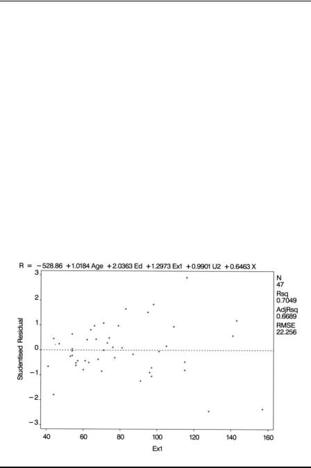
Having arrived at a final multiple regression model for a data set, it is important to go further and check the assumptions made in the modelling process. Most useful at this stage is an examination of residuals from the fitted model, along with many other regression diagnostics now available. Residuals at their simplest are the difference between the observed and fitted values of the response variable — in our example, crime rate. The most useful ways of examining the residuals are graphical, and the most useful plots are

A plot of the residuals against each explanatory variable in the model; the presence of a curvilinear relationship, for example, would suggest that a higher-order term (e.g., a quadratic) in the explanatory variable is needed in the model.

A plot of the residuals against predicted values of the response variable; if the variance of the response appears to increase with the predicted value, a transformation of the response may be in order.

A normal probability plot of the residuals; after all systematic variation has been removed from the data, the residuals should look like a sample from the normal distribution. A plot of the ordered residuals against the expected order statistics from a normal distribution provides a graphical check of this assumption.

Unfortunately, the simple observed-fitted residuals have a distribution that is scale dependent (see Cook and Weisberg [1982]), which makes them less helpful than they might be. The problem can be overcome, however,

©2002 CRC Press LLC

by using standardised or studentised residuals (both are explicitly defined in Cook and Weisberg [1982]) .

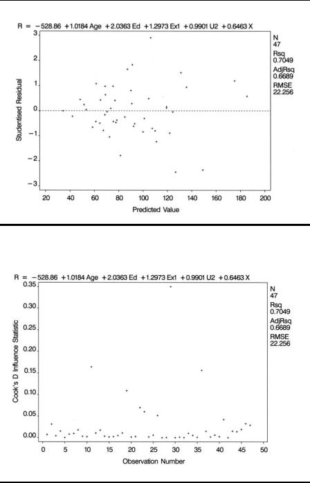
A variety of other diagnostics for regression models have been developed in the past decade or so. One that is often used is the Cook’s distance statistic (Cook [1977; 1979]). This statistic can be obtained for each of the n observations and measures the change to the estimates of the regression coefficients that would result from deleting the particular observation. It can be used to identify any observations having an undue influence of the estimation and fitting process.

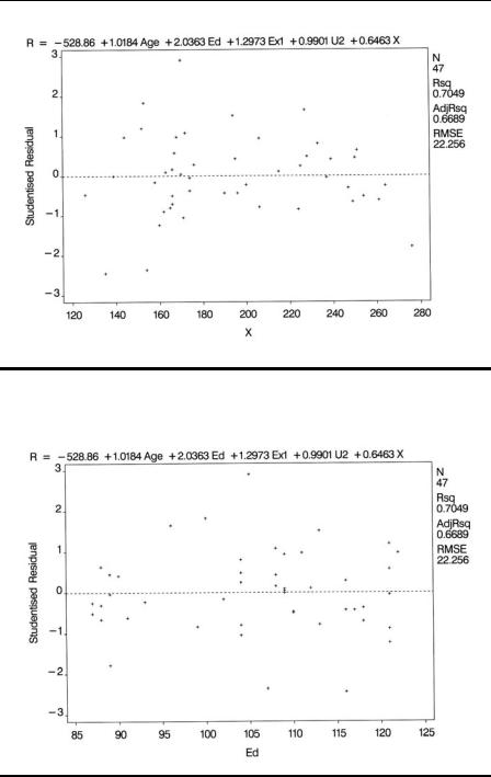
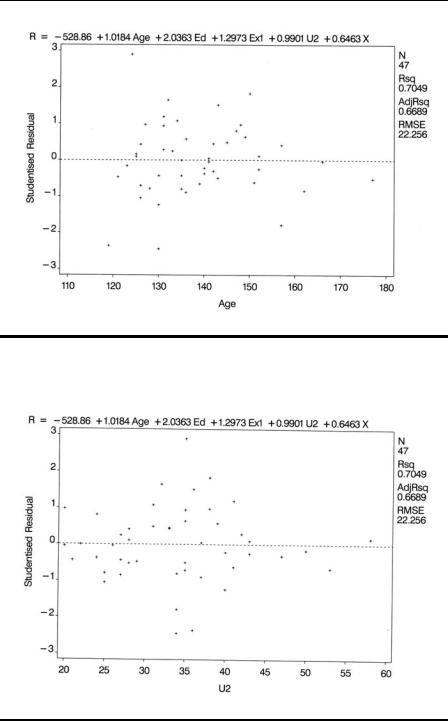
Plots of residuals and other diagnostics can be found using the plot statement to produce high-resolution diagnostic plots. Variables mentioned in the model or var statements can be plotted along with diagnostic statistics. The latter are represented by keywords that end in a period. The first plot statement produces plots of the studentised residual against the five predictor variables. The results are shown in Display 4.6 through Display 4.10. The next plot statement produces a plot of the studentised residuals against the predicted values and an index plot of Cook’s distance statistic. The resulting plots are shown in Displays 4.11 and 4.12. The final plot statement specifies a normal probability plot of the residuals, which is shown in Display 4.13.

Display 4.6

©2002 CRC Press LLC

Display 4.7

Display 4.8

©2002 CRC Press LLC

Display 4.9

Display 4.10

©2002 CRC Press LLC

Display 4.11

Display 4.12

©2002 CRC Press LLC

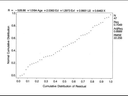
Display 4.13

Display 4.6 suggests increasing variability of the residuals with increasing values of Ex1. And Display 4.13 indicates a number of relatively large values for the Cook’s distance statistic although there are no values greater than 1, which is the usually accepted threshold for concluding that the corresponding observation has undue influence on the estimated regression coefficients.

Exercises

4.1Find the subset of five variables considered by the Cp option to be optimal. How does this subset compare with that chosen by the stepwise option?

4.2Apply the Cp criterion to exploring all possible subsets of the five variables chosen by the stepwise procedure (see Display 4.5). Produce a plot of the number of variables in a subset against the corresponding value of Cp.

4.3Examine some of the other regression diagnostics available with proc reg on the U.S. crime rate data.

4.4In the text, the problem of the high variance inflation factors associated with variables Ex0 and Ex1 was dealt with by excluding

©2002 CRC Press LLC

Ex0. An alternative is to use the average of the two variables as an explanatory variable. Investigate this possibility.

4.5Investigate the regression of crime rate on the two variables Age and S. Consider the possibility of an interaction of the two variables in the regression model, and construct some plots that illustrate the models fitted.

©2002 CRC Press LLC

Chapter 5

Analysis of Variance I:

Treating Hypertension

5.1 Description of Data

Maxwell and Delaney (1990) describe a study in which the effects of three possible treatments for hypertension were investigated. The details of the treatments are as follows:

All 12 combinations of the three treatments were included in a 3 × 2 × 2 design. Seventy-two subjects suffering from hypertension were recruited to the study, with six being randomly allocated to each of 12 treatment combinations. Blood pressure measurements were made on each subject after treatment, leading to the data in Display 5.1.

©2002 CRC Press LLC

Display 5.1

Questions of interest concern differences in mean blood pressure for the different levels of the three treatments and the possibility of interactions between the treatments.

5.2 Analysis of Variance Model

A possible model for these data is

yijkl = µ + α i + β j + γ k + (αβ )ij + (αγ )ik + (βγ )jk + (αβγ )ijk + ijkl (5.1)

where yijkl represents the blood pressure of the lth subject for the ith drug, the jth level of biofeedback, and the kth level of diet; µ is the overall mean; α i, β j, and γ k are the main effects of drugs, biofeedback, and diets; (αβ )ij, (αγ )ik, and (βγ )jk are the first-order interaction terms between pairs of treatments, (αβγ )ijk represents the second-order interaction term of the three treatments; and ijkl represents the residual or error terms assumed to be normally distributed with zero mean and variance σ 2. (The model as specified is over-parameterized and the parameters have to be constrained in some way, commonly by requiring them to sum to zero or setting one parameter at zero; see Everitt [2001] for details.)

Such a model leads to a partition of the variation in the observations into parts due to main effects, first-order interactions between pairs of factors, and a second-order interaction between all three factors. This partition leads to a series of F-tests for assessing the significance or otherwise of these various components. The assumptions underlying these F-tests include:

©2002 CRC Press LLC

The observations are independent of one another.

The observations in each cell arise from a population having a normal distribution.

The observations in each cell are from populations having the same variance.

5.3Analysis Using SAS

It is assumed that the 72 blood pressure readings shown in Display 5.1 are in the ASCII file hypertension.dat. The SAS code used for reading and labelling the data is as follows:

data hyper;

infile 'hypertension.dat'; input n1-n12;

if _n_<4 then biofeed='P'; else biofeed='A';

if _n_ in(1,4) then drug='X'; if _n_ in(2,5) then drug='Y'; if _n_ in(3,6) then drug='Z'; array nall {12} n1-n12;

do i=1 to 12;

if i>6 then diet='Y'; else diet='N'; bp=nall{i}; cell=drug||biofeed||diet; output;

end;

drop i n1-n12; run;

The 12 blood pressure readings per row, or line, of data are read into variables n1 - n12 and used to create 12 separate observations. The row and column positions in the data are used to determine the values of the factors in the design: drug, biofeed, and diet.

First, the input statement reads the 12 blood pressure values into variables n1 to n2. It uses list input, which assumes the data values to be separated by spaces.

The next group of statements uses the SAS automatic variable _n_ to determine which row of data is being processed and hence to set the

©2002 CRC Press LLC