

Handbook_of_statistical_analysis_using_SAS
.pdfSummary Statistics for Time Variable days
|
The LIFETEST Procedure |
|
||
|
Quartile Estimates |
|
||
|
Point |
95% Confidence Interval |
||
Percent |
Estimate |
(Lower) |
(Upper) |
|
75 |
580.00 |
464 |
.00 |
. |
50 |
254.00 |
193 |
.00 |
484.00 |
25 |
144.00 |
74 |
.00 |
195.00 |
Mean Standard Error
491.84 71.01
NOTE: The mean survival time and its standard error were underestimated because the largest observation was censored and the estimation was restricted to the largest event time.
|
|
The LIFETEST Procedure |
|
|
||
|
|
|
Stratum 2: group = 1 |
|
|
|
|
|
Product-Limit Survival Estimates |
|
|||
|
|
|
|
Survival |
|
|
|
|
|
|
Standard |
Number |
Number |
Days |
Survival |
Failure |
Error |
Failed |
Left |
|
0 |
.00 |
1.0000 |
0 |
0 |
0 |
44 |
1 |
.00 |
0.9773 |
0.0227 |
0.0225 |
1 |
43 |
63 |
.00 |
0.9545 |
0.0455 |
0.0314 |
2 |
42 |
105 |
.00 |
0.9318 |
0.0682 |
0.0380 |
3 |
41 |
125 |
.00 |
0.9091 |
0.0909 |
0.0433 |
4 |
40 |
182 |
.00 |
0.8864 |
0.1136 |
0.0478 |
5 |
39 |
216 |
.00 |
0.8636 |
0.1364 |
0.0517 |
6 |
38 |
250 |
.00 |
0.8409 |
0.1591 |
0.0551 |
7 |
37 |
262 |
.00 |
0.8182 |
0.1818 |
0.0581 |
8 |
36 |
301 |
.00 |
. |
. |
. |
9 |
35 |
301 |
.00 |
0.7727 |
0.2273 |
0.0632 |
10 |
34 |
342 |
.00 |
0.7500 |
0.2500 |
0.0653 |
11 |
33 |
354 |
.00 |
0.7273 |
0.2727 |
0.0671 |
12 |
32 |
356 |
.00 |
0.7045 |
0.2955 |
0.0688 |
13 |
31 |
358 |
.00 |
0.6818 |
0.3182 |
0.0702 |
14 |
30 |
380 |
.00 |
0.6591 |
0.3409 |
0.0715 |
15 |
29 |
383 |
.00 |
. |
. |
. |
16 |
28 |
©2002 CRC Press LLC

383 |
.00 |
0.6136 |
0.3864 |
0.0734 |
17 |
27 |
388 |
.00 |
0.5909 |
0.4091 |
0.0741 |
18 |
26 |
394 |
.00 |
0.5682 |
0.4318 |
0.0747 |
19 |
25 |
408 |
.00 |
0.5455 |
0.4545 |
0.0751 |
20 |
24 |
460 |
.00 |
0.5227 |
0.4773 |
0.0753 |
21 |
23 |
489 |
.00 |
0.5000 |
0.5000 |
0.0754 |
22 |
22 |
523 |
.00 |
0.4773 |
0.5227 |
0.0753 |
23 |
21 |
524 |
.00 |
0.4545 |
0.5455 |
0.0751 |
24 |
20 |
535 |
.00 |
0.4318 |
0.5682 |
0.0747 |
25 |
19 |
562 |
.00 |
0.4091 |
0.5909 |
0.0741 |
26 |
18 |
569 |
.00 |
0.3864 |
0.6136 |
0.0734 |
27 |
17 |
675 |
.00 |
0.3636 |
0.6364 |
0.0725 |
28 |
16 |
676 |
.00 |
0.3409 |
0.6591 |
0.0715 |
29 |
15 |
748 |
.00 |
0.3182 |
0.6818 |
0.0702 |
30 |
14 |
778 |
.00 |
0.2955 |
0.7045 |
0.0688 |
31 |
13 |
786 |
.00 |
0.2727 |
0.7273 |
0.0671 |
32 |
12 |
797 |
.00 |
0.2500 |
0.7500 |
0.0653 |
33 |
11 |
955 |
.00 |
0.2273 |
0.7727 |
0.0632 |
34 |
10 |
968 |
.00 |
0.2045 |
0.7955 |
0.0608 |
35 |
9 |
977 |
.00 |
0.1818 |
0.8182 |
0.0581 |
36 |
8 |
1245 |
.00 |
0.1591 |
0.8409 |
0.0551 |
37 |
7 |
1271 |
.00 |
0.1364 |
0.8636 |
0.0517 |
38 |
6 |
1420 |
.00 |
0.1136 |
0.8864 |
0.0478 |
39 |
5 |
1460.00* |
. |
. |
. |
39 |
4 |
|
1516.00* |
. |
. |
. |
39 |
3 |
|
1551 |
.00 |
0.0758 |
0.9242 |
0.0444 |
40 |
2 |
1690.00* |
. |
. |
. |
40 |
1 |
|
1694 |
.00 |
0 |
1.0000 |
0 |
41 |
0 |
NOTE: The marked survival times are censored observations.
Summary Statistics for Time Variable days
|
Quartile Estimates |
|
|
|
|
Point |
95% Confidence Interval |
||
Percent |
Estimate |
(Lower) |
(Upper) |
|
75 |
876.00 |
569.00 |
1271 |
.00 |
50 |
506.00 |
383.00 |
676 |
.00 |
25 |
348.00 |
250.00 |
388 |
.00 |
The LIFETEST Procedure
Mean Standard Error
653.22 72.35
©2002 CRC Press LLC

Summary of the Number of Censored and Uncensored Values
|
|
|
|
|
Percent |
Stratum |
group |
Total |
Failed |
Censored |
Censored |
1 |
0 |
45 |
38 |
7 |
5.56 |
2 |
1 |
44 |
41 |
3 |
6.82 |
-------------------------------------------------------------------------------
Total |
89 |
79 |
10 |
11.24 |
The LIFETEST Procedure
Testing Homogeneity of Survival Curves for days over Strata
|
Rank Statistics |
|
||
group |
Log-Rank |
Wilcoxon |
||
0 |
3 |
.3043 |
502 |
.00 |
1 |
-3 |
.3043 |
-502 |
.00 |
Covariance Matrix for the Log-Rank Statistics
group |
|
0 |
|
1 |
0 |
19 |
.3099 |
-19 |
.3099 |
1 |
-19 |
.3099 |
19 |
.3099 |
Covariance Matrix for the Wilcoxon Statistics
group |
|
0 |
|
|
1 |
0 |
58385 |
.0 |
-58385 |
.0 |
|
1 |
-58385 |
.0 |
58385 |
.0 |
|
Test of Equality over Strata |
|||||
|
|
|
|
|
Pr > |
Test |
Chi-Square |
DF |
Chi-Square |
||
Log-Rank |
0.5654 |
1 |
|
0.4521 |
|
Wilcoxon |
4.3162 |
1 |
|
0.0378 |
|
-2Log(LR) |
0.3574 |
1 |
|
0.5500 |
|
Display 12.4
©2002 CRC Press LLC
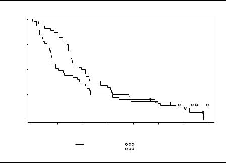
Survival Distribution Function
1.00
0.75
0.50
0.25
0.00
0 |
250 |
500 |
750 |
1000 |
1250 |
1500 |
1750 |
|
|
|
|
days |
|
|
|
|
STRATA: |
group= 0 |
|
Censored group= 0 |
|
|
|
|
|
group= 1 |
|
Censored group= 1 |
|
|
|
Display 12.5
12.3.2 Methadone Treatment of Heroin Addicts
The data on treatment of heroin addiction shown in Display 12.2 can be read in with the following data step.
data heroin;
infile 'n:\handbook2\datasets\heroin.dat' expandtabs; input id clinic status time prison dose @@;
run;
Each line contains the data values for two observations, but there is no relevant difference between those that occur first and second. This being the case, the data can be read using list input and a double trailing @. This holds the current line for further data to be read from it. The difference between the double trailing @ and the single trailing @, used for the cancer data, is that the double @ will hold the line across iterations of the data step. SAS will only go on to a new line when it runs out of data on the current line.
©2002 CRC Press LLC
The SAS log will contain the message "NOTE: SAS went to a new line when INPUT statement reached past the end of a line," which is not a cause for concern in this case. It is also worth noting that although the ID variable ranges from 1 to 266, there are actually 238 observations in the data set.
Cox regression is implemented within SAS in the phreg procedure. The data come from two different clinics and it is possible, indeed
likely, that these clinics have different hazard functions which may well not be parallel. A Cox regression model with clinics as strata and the other two variables, dose and prison, as explanatory variables can be fitted in SAS using the phreg procedure.
proc phreg data=heroin;
model time*status(0)=prison dose / rl; strata clinic;
run;
In the model statement, the response variable (i.e., the failure time) is followed by an asterisk, the name of the censoring variable, and a list of censoring value(s) in parentheses. As with proc reg, the predictors must all be numeric variables. There is no built-in facility for dealing with categorical predictors, interactions, etc. These must all be calculated as separate numeric variables and dummy variables.
The rl (risklimits) option requests confidence limits for the hazard ratio. By default, these are the 95% limits.
The strata statement specifies a stratified analysis with clinics forming the strata.
The output is shown in Display 12.6. Examining the maximum likelihood estimates, we find that the parameter estimate for prison is 0.38877 and that for dose –0.03514. Interpretation becomes simpler if we concentrate on the exponentiated versions of those given under Hazard Ratio. Using the approach given in Eq. (12.13), we see first that subjects with a prison history are 47.5% more likely to complete treatment than those without a prison history. And for every increase in methadone dose by one unit (1mg), the hazard is multiplied by 0.965. This coefficient is very close to 1, but this may be because 1 mg methadone is not a large quantity. In fact, subjects in this study differ from each other by 10 to 15 units, and thus it may be more informative to find the hazard ratio of two subjects differing by a standard deviation unit. This can be done simply by rerunning the analysis with the dose standardized to zero mean and unit variance;
©2002 CRC Press LLC

|
|
The PHREG Procedure |
|
||
|
|
Model Information |
|
||
|
Data Set |
WORK.HEROIN |
|
||
|
Dependent Variable |
time |
|
||
|
Censoring Variable |
status |
|
||
|
Censoring Value(s) |
0 |
|
|
|
|
Ties Handling |
BRESLOW |
|
||
Summary of the Number of Event and Censored Values |
|||||
|
|
|
|
|
Percent |
Stratum |
clinic |
Total Event |
Censored |
Censored |
|
1 |
1 |
163 |
122 |
41 |
25.15 |
2 |
2 |
75 |
28 |
47 |
62.67 |
---------------------------------------------------------------------------
Total |
238 |
150 |
88 |
36.97 |
Convergence Status
Convergence criterion (GCONV=1E-8) satisfied.
Model Fit Statistics
|
Without |
|
With |
|
Criterion |
Covariates |
Covariates |
||
-2 LOG L |
1229 |
.367 |
1195.428 |
|
AIC |
1229 |
.367 |
1199.428 |
|
SBC |
1229 |
.367 |
1205.449 |
|
Testing Global Null Hypothesis: BETA=0 |
||||
Test |
Chi-Square |
DF |
Pr > ChiSq |
|
Likelihood Ratio |
33.9393 |
2 |
<.0001 |
|
Score |
33.3628 |
2 |
<.0001 |
|
Wald |
32.6858 |
2 |
<.0001 |
|
©2002 CRC Press LLC

Analysis of Maximum Likelihood Estimates
|
|
Parameter |
Standard |
|
Chi- |
Pr > |
Hazard |
95% Hazard Ratio |
||
Variable |
DF |
Estimate |
Error |
Square |
ChiSq |
Ratio |
Confidence |
Limits |
||
prison |
1 |
0 |
.38877 |
0.16892 |
5 |
.2974 |
0.0214 |
1.475 |
1.059 |
2.054 |
dose |
1 |
-0 |
.03514 |
0.00647 |
29 |
.5471 |
<.0001 |
0.965 |
0.953 |
0.978 |
Display 12.6
The analysis can be repeated with dose standardized to zero mean and unit variance as follows:
proc stdize data=heroin out=heroin2; var dose;
proc phreg data=heroin2;
model time*status(0)=prison dose / rl; strata clinic;
baseline out=phout loglogs=lls / method=ch;
symbol1 i=join v=none l=1; symbol2 i=join v=none l=3; proc gplot data=phout;
plot lls*time=clinic; run;
The stdize procedure is used to standardize dose (proc standard could also have been used). Zero mean and unit variance is the default method of standardization. The resulting data set is given a different name with the out= option and the variable to be standardized is specified with the var statement.
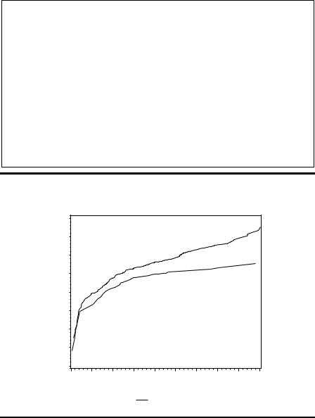
The phreg step uses this new data set to repeat the analysis. The baseline statement is added to save the log cumulative hazards in the data set phout. loglogs=lls specifies that the log of the negative log of survival is to be computed and stored in the variable lls. The product limit estimator is the default and method=ch requests the alternative empirical cumulative hazard estimate.
Proc gplot is then used to plot the log cumulative hazard with the symbol statements defining different linetypes for each clinic.
©2002 CRC Press LLC

The output from the phreg step is shown in Display 12.7 and the plot in Display 12.8. The coefficient of dose is now –0.50781 and the hazard ratio is 0.602. This can be interpreted as indicating a decrease in the hazard by 40% when the methadone dose increases by one standard deviation unit. Clearly, an increase in methadone dose decreases the likelihood of the addict completing treatment.
In Display 12.8, the increment at each event represents the estimated logs of the hazards at that time. Clearly, the curves are not parallel, underlying that treating the clinics as strata was sensible.
|
|
The PHREG Procedure |
|
||
|
|
Model Information |
|
||
|
Data Set |
WORK.HEROIN2 |
|
||
|
Dependent Variable |
time |
|
|
|
|
Censoring Variable |
status |
|
||
|
Censoring Value(s) |
0 |
|
|
|
|
Ties Handling |
BRESLOW |
|
||
Summary of the Number of Event and Censored Values |
|||||
|
|
|
|
|
Percent |
Stratum |
Clinic |
Total Event |
Censored |
Censored |
|
1 |
1 |
163 |
122 |
41 |
25.15 |
2 |
2 |
75 |
28 |
47 |
62.67 |
---------------------------------------------------------------------------
Total |
238 |
150 |
88 |
36.97 |
Convergence Status
Convergence criterion (GCONV=1E-8) satisfied.
Model Fit Statistics
|
Without |
With |
Criterion |
Covariates |
Covariates |
-2 LOG L |
1229.367 |
1195.428 |
AIC |
1229.367 |
1199.428 |
SBC |
1229.367 |
1205.449 |
©2002 CRC Press LLC
Testing Global Null Hypothesis: BETA=0
Test |
Chi-Square |
DF |
Pr > ChiSq |
Likelihood Ratio |
33.9393 |
2 |
<.0001 |
Score |
33.3628 |
2 |
<.0001 |
Wald |
32.6858 |
2 |
<.0001 |
Analysis of Maximum Likelihood Estimates
|
|
Parameter |
Standard |
|
Chi- |
Pr > |
Hazard |
95% Hazard Ratio |
||
Variable |
DF |
Estimate |
Error |
Square |
ChiSq |
Ratio |
Confidence Limits |
|||
prison |
1 |
0 |
.38877 |
0.16892 |
5 |
.2974 |
0.0214 |
1.475 |
1.059 |
2.054 |
dose |
1 |
-0 |
.50781 |
0.09342 |
29 |
.5471 |
<.0001 |
0.602 |
0.501 |
0.723 |
Display 12.7
Log of Negative Log of SURVIVAL
2
1
0
-1
-2
-3
-4
-5
-6
0 |
100 |
200 |
300 |
400 |
500 |
600 |
700 |
800 |
900 |
|
|
|
|
|
|
|
time |
|
|
|
|
|
clinic |
|
|
1 |
2 |
|
|
|
|
|
|
|
|
|
|
|
|
|
|||
Display 12.8
©2002 CRC Press LLC

Exercises
12.1In the original analyses of the data in this chapter (see Caplehorn and Bell, 1991), it was judged that the hazards were approximately proportional for the first 450 days (see Display 12.8). Consequently, the data for this time period were analysed using clinic as a covariate rather than by stratifying on clinic. Repeat this analysis using clinic, prison, and standardized dose as covariates.
12.2Following Caplehorn and Bell (1991), repeat the analyses in Exercise
12.1 but now treating dose as a categorical variable with three levels (<60, 60–79, ≥ 80) and plot the predicted survival curves for the three dose categories when prison takes the value 0 and clinic the value 1.
12.3Test for an interaction between clinic and methadone using both continuous and categorical scales for dose.
12.4Investigate the use of residuals in fitting a Cox regression using some of the models fitted in the text and in the previous exercises.
©2002 CRC Press LLC