Handbook_of_statistical_analysis_using_SAS

Note: F: Female, M: Male.

Display 8.1

The third data set is given in Display 8.3 and results from asking a sample of employed men, ages 18 to 67, whether, in the preceding year, they had carried out work in their home that they would have previously employed a craftsman to do. The response variable here is the answer (yes/no) to that question. In this situation, we would like to model the relationship between the response variable and four categorical explanatory variables: work, tenure, accommodation type, and age.

©2002 CRC Press LLC

3.3235 0

Display 8.2

©2002 CRC Press LLC

Display 8.3

8.2 The Logistic Regression Model

In linear regression (see Chapter 3), the expected value of a response variable y is modelled as a linear function of the explanatory variables:

For a dichotomous response variable coded 0 and 1, the expected value is simply the probability π that the variable takes the value 1. This could be modelled as in Eq. (8.1), but there are two problems with using linear regression when the response variable is dichotomous:

1.The predicted probability must satisfy 0 ≤ π ≤ 1, whereas a linear predictor can yield any value from minus infinity to plus infinity.

2.The observed values of y do not follow a normal distribution with mean π , but rather a Bernoulli (or binomial [1, π ]) distribution.

In logistic regression, the first problem is addressed by replacing the probability π = E(y) on the left-hand side of Eq. (8.1) with the logit transformation of the probability, log π /(1 – π ). The model now becomes:

©2002 CRC Press LLC

The logit of the probability is simply the log of the odds of the event of interest. Setting β ′ = [β 0, β 1, …, β p] and the augmented vector of scores for the ith individual as xi′ = [1, xi1, xi2, …, xip], the predicted probabilities as a function of the linear predictor are:

Whereas the logit can take on any real value, this probability always satisfies 0 ≤ π (β′ xi) ≤ 1. In a logistic regression model, the parameter β i associated with explanatory variable xi is such that exp(β i) is the odds that y = 1 when xi increases by 1, conditional on the other explanatory variables remaining the same.

Maximum likelihood is used to estimate the parameters of Eq. (8.2), the log-likelihood function being:

where y′ = [y1, y2, …, yn] are the n observed values of the dichotomous response variable. This log-likelihood is maximized numerically using an iterative algorithm. For full details of logistic regression, see, for example, Collett (1991).

8.3 Analysis Using SAS

8.3.1 GHQ Data

Assuming the data are in the file 'ghq.dat'in the current directory and that the data values are separated by tabs, they can be read in as follows:

data ghq;

infile 'ghq.dat' expandtabs; input ghq sex $ cases noncases; total=cases+noncases; prcase=cases/total;

run;

©2002 CRC Press LLC

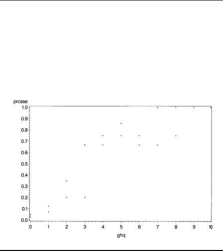
The variable prcase contains the observed probability of being a case. This can be plotted against ghq score as follows:

proc gplot data=ghq; plot prcase*ghq;

run;

The resulting plot is shown in Display 8.4. Clearly, as the GHQ score increases, the probability of being considered a case increases.

Display 8.4

It is a useful exercise to compare the results of fitting both a simple linear regression and a logistic regression to these data using the single explanatory variable GHQ score. First we perform a linear regression using proc reg:

proc reg data=ghq; model prcase=ghq;

output out=rout p=rpred; run;

The output statement creates an output data set that contains all the original variables plus those created by options. The p=rpred option specifies that

©2002 CRC Press LLC

the predicted values are included in a variable named rpred. The out=rout option specifies the name of the data set to be created.

We then calculate the predicted values from a logistic regression, using proc logistic, in the same way:

proc logistic data=ghq; model cases/total=ghq; output out=lout p=lpred;

run;

There are two forms of model statement within proc logistic. This example shows the events/trials syntax, where two variables are specified separated by a slash. The alternative is to specify a single binary response variable before the equal sign.

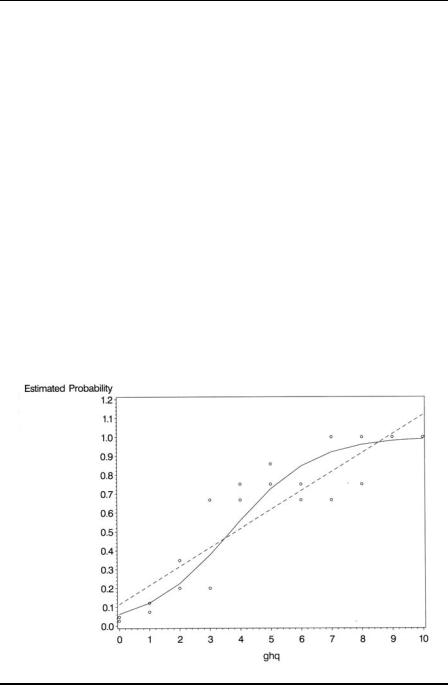
The two output data sets are combined in a short data step. Because proc gplot plots the data in the order in which they occur, if the points are to be joined by lines it may be necessary to sort the data set into the appropriate order. Both sets of predicted probabilities are to be plotted on the same graph (Display 8.5), together with the observed values; thus, three symbol statements are defined to distinguish them:

Display 8.5

©2002 CRC Press LLC

data lrout; set rout; set lout;

proc sort data=lrout; by ghq;

symbol1 i=join v=none l=1; symbol2 i=join v=none l=2; symbol3 v=circle;

proc gplot data=lrout;

plot (rpred lpred prcase)*ghq /overlay; run;

The problems of using the unsuitable linear regression model become apparent on studying Display 8.5. Using this model, two of the predicted values are greater than 1, but the response is a probability constrained to be in the interval (0,1). Additionally, the model provides a very poor fit for the observed data. Using the logistic model, on the other hand, leads to predicted values that are satisfactory in that they all lie between 0 and 1, and the model clearly provides a better description of the observed data.

Next we extend the logistic regression model to include both ghq score and sex as explanatory variables:

proc logistic data=ghq; class sex;

model cases/total=sex ghq; run;

The class statement specifies classification variables, or factors, and these can be numeric or character variables. The specification of explanatory effects in the model statement is the same as for proc glm:, with main effects specified by variable names and interactions by joining variable names with asterisks. The bar operator can also be used as an abbreviated way of entering interactions if these are to be included in the model (see Chapter 5).

The output is shown in Display 8.6. The results show that the estimated parameters for both sex and GHQ are significant beyond the 5% level. The parameter estimates are best interpreted if they are converted into odds ratios by exponentiating them. For GHQ, for example, this leads to

©2002 CRC Press LLC

an odds ratio estimate of exp(0.7791) (i.e., 2.180), with a 95% confidence interval of (1.795, 2.646). A unit increase in GHQ increases the odds of being a case between about 1.8 and 3 times, conditional on sex.

The same procedure can be applied to the parameter for sex, but more care is needed here because the Class Level Information in Display 8.5 shows that sex is coded 1 for females and –1 for males. Consequently, the required odds ratio is exp(2 × 0.468) (i.e., 2.55), with a 95% confidence interval of (1.088, 5.974). Being female rather than male increases the odds of being a case between about 1.1 and 6 times, conditional on GHQ.

The LOGISTIC Procedure

Model Information

Model Convergence Status

Convergence criterion (GCONV=1E-8) satisfied.

Model Fit Statistics

©2002 CRC Press LLC

Testing Global Null Hypothesis: BETA=0

Type III Analysis of Effects

The LOGISTIC Procedure

Analysis of Maximum Likelihood Estimates

©2002 CRC Press LLC

Association of Predicted Probabilities and Observed Responses

Display 8.6

8.3.2 ESR and Plasma Levels

We now move on to examine the ESR data in Display 8.2. The data are first read in for analysis using the following SAS code:

data plasma;

infile 'n:\handbook2\datasets\plasma.dat'; input fibrinogen gamma esr;

run;

We can try to identify which of the two plasma proteins — fibrinogen or γ -globulin — has the strongest relationship with ESR level by fitting a logistic regression model and allowing here, backward elimination of variables as described in Chapter 3 for multiple regression, although the elimination criterion is now based on a likelihood ratio statistic rather than an F-value.

proc logistic data=plasma desc;

model esr=fibrinogen gamma fibrinogen*gamma / selection=backward;

run;

Where a binary response variable is used on the model statement, as opposed to the events/trials used for the GHQ data, SAS models the lower of the two response categories as the “event.” However, it is common practice for a binary response variable to be coded 0,1 with 1 indicating a response (or event) and 0 indicating no response (or a non-event). In this case, the seemingly perverse, default in SAS will be to model the probability of a non-event. The desc (descending) option in the proc statement reverses this behaviour.

It is worth noting that when the model selection option is forward, backward, or stepwise, SAS preserves the hierarchy of effects by default.

©2002 CRC Press LLC