Handbook_of_statistical_analysis_using_SAS

Display 10.3

The data are first sorted by group and time within group. To use the by statement to produce separate box plots for each group, the data must be sorted by group. Proc boxplot also requires the data to be sorted by the x-axis variable, time in this case. The results are shown in Displays 10.4 and 10.5. Again, the decline in depression scores in both groups is clearly seen in the graphs.

goptions reset=symbol; symbol1 i=stdm1j l=1; symbol2 i=stdm1j l=2; proc gplot data=pndep2;

plot dep*time=group; run;

The goptions statement resets symbols to their defaults and is recommended when redefining symbol statements that have been previously used in the same session. The std interpolation option can be used to plot means and their standard deviations for data where multiple values of y occur for each value of x: std1, std2, and std3 result in a line 1, 2, and 3 standard deviations above and below the mean. Where m is suffixed,

©2002 CRC Press LLC

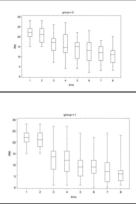
Display 10.4

Display 10.5

©2002 CRC Press LLC

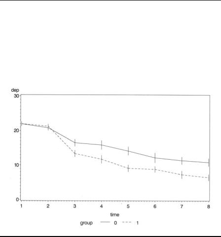
as here, it is the standard error of the mean that is used. The j suffix specifies that the means should be joined. There are two groups in the data, so two symbol statements are used with different l (linetype) options to distinguish them. The result is shown in Display 10.6, which shows that from the first visit after randomisation (time 3), the depression score in the active group is lower than in the control group, a situation that continues for the remainder of the trial.

Display 10.6

The scatterplot matrix is produced using the scattmat SAS macro introduced in Chapter 4 and listed in Appendix A. The result is shown in Display 10.7. Clearly, observations made on occasions close together in time are more strongly related than those made further apart, a phenomenon that may have implications for more formal modelling of the data (see Chapter 11).

%include 'scattmat.sas'; %scattmat(pndep,x1-x8);

©2002 CRC Press LLC

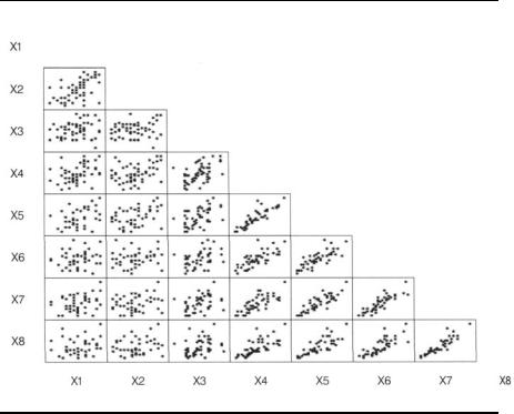
Display 10.7

10.3.2Response Feature Analysis

A relatively straightforward approach to the analysis of longitudinal data is that involving the use of summary measures, sometimes known as response feature analysis. The repeated observations on a subject are used to construct a single number that characterises some relevant aspect of the subject’s response profile. (In some situations, more than a single summary measure may be needed to characterise the profile adequately.) The summary measure to be used does, of course, need to be decided upon prior to the analysis of the data.

The most commonly used summary measure is the mean of the responses over time because many investigations (e.g., clinical trials) are most concerned with differences in overall level rather than more subtle effects. However, other summary measures might be considered more relevant in particular circumstances, and Display 10.8 lists a number of alternative possibilities.

©2002 CRC Press LLC

Having identified a suitable summary measure, the analysis of the repeated measures data reduces to a simple univariate test of group differences on the chosen measure. In the case of two groups, this will involve the application of a two-sample t-test or perhaps its nonparametric equivalent.

Returning to the oestrogen patch data, we will use the mean as the chosen summary measure, but there are two further problems to consider:

1.How to deal with the missing values

2.How to incorporate the pretreatment measurements into an analysis

The missing values can be dealt with in at least three ways:

1.Take the mean over the available observations for a subject; that is, if a subject has only four post-treatment values recorded, use the mean of these.

©2002 CRC Press LLC

2.Include in the analysis only those subjects with all six posttreatment observations.

3.Impute the missing values in some way; for example, use the last observation carried forward (LOCF) approach popular in the pharmaceutical industry.

The pretreatment values might be incorporated by calculating change scores, that is, post-treatment mean – pretreatment mean value, or as covariates in an analysis of covariance of the post-treatment means. Let us begin, however, by simply ignoring the pretreatment values and deal only with the post-treatment means.

The three possibilities for calculating the mean summary measure can be implemented as follows:

data pndep; set pndep;

array xarr {8} x1-x8; array locf {8} locf1-locf8; do i=3 to 8;

locf{i}=xarr{i};

if xarr{i}=. then locf{i}=locf{i-1}; end;

mnbase=mean(x1,x2); mnresp=mean(of x3-x8); mncomp=(x3+x4+x5+x6+x7+x8)/6; mnlocf=mean(of locf3-locf8); chscore=mnbase-mnresp;

run;

The summary measures are to be included in the pndep data set, so this is named in the data statement. The set statement indicates that the data are to be read from the current version of pndep. The eight depression scores x1-x8 are declared as an array and another array is declared for the LOCF values. Eight variables are declared, although only six will be used. The do loop assigns LOCF values for those occasions when the depression score was missing. The mean of the two baseline measures is then computed using the SAS mean function. The next statement computes the mean of the recorded follow-up scores. When a variable list is used with the mean function, it must be preceded with 'of'. The mean function will only result in a missing value if all the variables are missing. Otherwise, it computes the mean of the non-missing values. Thus, the mnresp variable will contain the mean of the available follow-up

©2002 CRC Press LLC

scores for a subject. Because an arithmetic operation involving a missing value results in a missing value, mncomp will be assigned a missing value if any of the variables is missing.

A t-test can now be applied to assess difference between treatments for each of the three procedures. The results are shown in Display 10.9.

proc ttest data=pndep; class group;

var mnresp mnlocf mncomp; run;

The TTEST Procedure

Statistics

Display 10.9

©2002 CRC Press LLC

Here, the results are similar and the conclusion in each case the same; namely, that there is a substantial difference in overall level in the two treatment groups. The confidence intervals for the treatment effect given by each of the three procedures are:

Using mean of available observations (1.612, 6.810)

Using LOCF (1.614, 6.987)

Using only complete cases (1.298, 6.851)

All three approaches lead, in this example, to the conclusion that the active treatment considerably lowers depression. But, in general, using only subjects with a complete set of measurements and last observation carried forward are not to be recommended. Using only complete observations can produce bias in the results unless the missing observations are missing completely at random (see Everitt and Pickles [1999]). And the LOCF procedure has little in its favour because it makes highly unlikely assumptions; for example, that the expected value of the (unobserved) remaining observations remain at their last recorded value. Even using the mean of the values actually recorded is not without its problems (see Matthews [1993]), but it does appear, in general, to be the least objectionable of the three alternatives.

Now consider analyses that make use of the pretreatment values available for each woman in the study. The change score analysis and the analysis of covariance using the mean of available post-treatment values as the summary and the mean of the two pretreatment values as covariate can be applied as follows:

proc glm data=pndep; class group;

model chscore=group /solution;

proc glm data=pndep; class group;

model mnresp=mnbase group /solution; run;

We use proc glm for both analyses for comparability, although we could also have used a t-test for the change scores. The results are shown in Display 10.10. In both cases for this example, the group effect is highly significant, confirming the difference in depression scores of the active and control group found in the previous analysis.

In general, the analysis of covariance approach is to be preferred for reasons outlined in Senn (1998) and Everitt and Pickles (2000).

©2002 CRC Press LLC

The GLM Procedure

Class Level Information

Class Levels Values

Number of observations 61

The GLM Procedure

Dependent Variable: chscore

©2002 CRC Press LLC

The GLM Procedure

Class Level Information

Class Levels Values

Number of observations 61

The GLM Procedure

Dependent Variable: mnresp

©2002 CRC Press LLC