Handbook_of_statistical_analysis_using_SAS

values of drug and biofeed. Because six lines of data will be read, one line per iteration of the data step _n_ will increment from 1 to 6, corresponding to the line of data read with the input statement.

The key elements in splitting the one line of data into separate observations are the array, the do loop, and the output statement. The array statement defines an array by specifying the name of the array (nall here), the number of variables to be included in braces, and the list of variables to be included (n1 to n12 in this case).

In SAS, an array is a shorthand way of referring to a group of variables. In effect, it provides aliases for them so that each variable can be referred to using the name of the array and its position within the array in braces. For example, in this data step, n12 could be referred to as nall{12} or, when the variable i has the value 12 as nall{i}. However, the array only lasts for the duration of the data step in which it is defined.

The main purpose of an iterative do loop, like the one used here, is to repeat the statements between the do and the end a fixed number of times, with an index variable changing at each repetition. When used to process each of the variables in an array, the do loop should start with the index variable equal to 1 and end when it equals the number of variables in the array.

Within the do loop, in this example, the index variable i is first used to set the appropriate values for diet. Then a variable for the blood pressure reading (bp) is assigned one of the 12 values input. A character variable (cell) is formed by concatenating the values of the drug, biofeed, and diet variables. The double bar operator (||) concatenates character values.

The output statement writes an observation to the output data set with the current value of all variables. An output statement is not normally necessary because, without it an observation is automatically written out at the end of the data step. Putting an output statement within the do loop results in 12 observations being written to the data set.

Finally, the drop statement excludes the index variable i and n1 to n12 from the output data set because they are no longer needed.

As with any relatively complex data manipulation, it is wise to check that the results are as they should be, for example, by using proc print.

To begin the analysis, it is helpful to look at some summary statistics for each of the cells in the design.

proc tabulate data=hyper; class drug diet biofeed; var bp;

table drug*diet*biofeed, bp*(mean std n);

run;

©2002 CRC Press LLC

The tabulate procedure is useful for displaying descriptive statistics in a concise tabular form. The variables used in the table must first be declared in either a class statement or a var statement. Class variables are those used to divide the observations into groups. Those declared in the var statement (analysis variables) are those for which descriptive statistics are to be calculated. The first part of the table statement up to the comma specifies how the rows of the table are to be formed, and the remaining part specifies the columns. In this example, the rows comprise a hierarchical grouping of biofeed within diet within drug. The columns comprise the blood pressure mean and standard deviation and cell count for each of the groups. The resulting table is shown in Display 5.2. The differences between the standard deviations seen in this display may have implications for the analysis of variance of these data because one of the assumptions made is that observations in each cell come from populations with the same variance.

Display 5.2

There are various ways in which the homogeneity of variance assumption can be tested. Here, the hovtest option of the anova procedure is used to apply Levene’s test (Levene [1960]). The cell variable calculated above, which has 12 levels corresponding to the 12 cells of the design, is used:

proc anova data=hyper; class cell;

©2002 CRC Press LLC

model bp=cell; means cell / hovtest;

run;

The results are shown in Display 5.3. Concentrating on the results of Levene’s test given in this display, we see that there is no formal evidence of heterogeneity of variance, despite the rather different observed standard deviations noted in Display 5.2.

©2002 CRC Press LLC

The ANOVA Procedure

Levene's Test for Homogeneity of bp Variance

ANOVA of Squared Deviations from Group Means

Display 5.3

To apply the model specified in Eq. (5.1) to the hypertension data, proc anova can now be used as follows:

proc anova data=hyper; class diet drug biofeed;

model bp=diet|drug|biofeed; means diet*drug*biofeed;

ods output means=outmeans; run;

The anova procedure is specifically for balanced designs, that is, those with the same number of observations in each cell. (Unbalanced designs should be analysed using proc glm, as illustrated in a subsequent chapter.) The class statement specifies the classification variables, or factors. These

©2002 CRC Press LLC

may be numeric or character variables. The model statement specifies the dependent variable on the left-hand side of the equation and the effects (i.e., factors and their interactions) on the right-hand side of the equation. Main effects are specified by including the variable name and interactions by joining the variable names with an asterisk. Joining variable names with a bar is a shorthand way of specifying an interaction and all the lower-order interactions and main effects implied by it. Thus, the model statement above is equivalent to:

model bp=diet drug diet*drug biofeed diet*biofeed drug*biofeed diet*drug*biofeed;

The order of the effects is determined by the expansion of the bar operator from left to right.

The means statement generates a table of cell means and the ods output statement specifies that this is to be saved in a SAS data set called outmeans.

The results are shown in Display 5.4. Here, it is the analysis of variance table that is of most interest. The diet, biofeed, and drug main effects are all significant beyond the 5% level. None of the first-order interactions are significant, but the three-way, second-order interaction of diet, drug, and biofeedback is significant. Just what does such an effect imply, and what are its implications for interpreting the analysis of variance results?

First, a significant second-order interaction implies that the first-order interaction between two of the variables differs in form or magnitude in the different levels of the remaining variable. Second, the presence of a significant second-order interaction means that there is little point in drawing conclusions about either the non-significant first-order interactions or the significant main effects. The effect of drug, for example, is not consistent for all combinations of diet and biofeedback. It would therefore be potentially misleading to conclude, on the basis of the significant main effect, anything about the specific effects of these three drugs on blood pressure.

The ANOVA Procedure

Class Level Information

©2002 CRC Press LLC

Display 5.4

©2002 CRC Press LLC

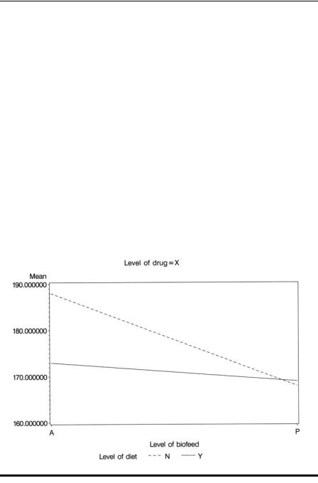
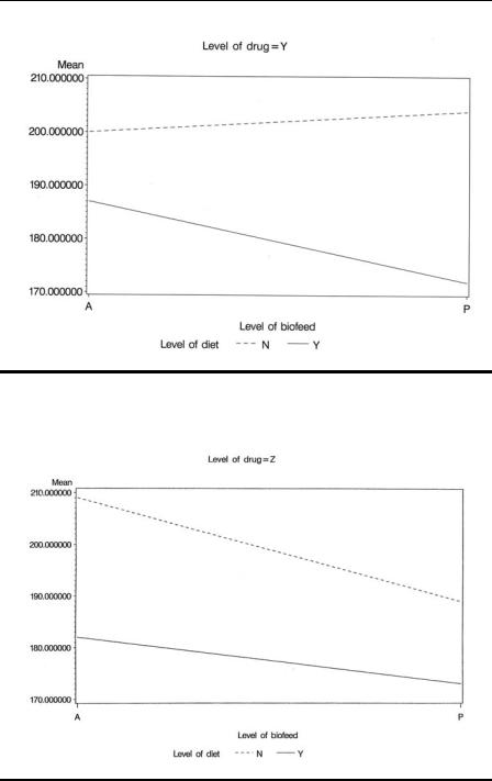
Understanding the meaning of the significant second-order interaction is facilitated by plotting some simple graphs. Here, the interaction plot of diet and biofeedback separately for each drug will help.

The cell means in the outmeans data set are used to produce interaction diagrams as follows:

proc print data=outmeans; proc sort data=outmeans;

by drug;

symbol1 i=join v=none l=2; symbol2 i=join v=none l=1;

proc gplot data=outmeans; plot mean_bp*biofeed=diet ; by drug;

run;

First the outmeans data set is printed. The result is shown in Display 5.5. As well as checking the results, this also shows the name of the variable containing the means.

To produce separate plots for each drug, we use the by statement within proc gplot, but the data set must first be sorted by drug. Plot statements of the form plot y*x=z were introduced in Chapter 1 along with the symbol statement to change the plotting symbols used. We know that diet has two values, so we use two symbol statements to control the way in which the means for each value of diet are plotted. The i (interpolation) option specifies that the means are to be joined by lines. The v (value) option suppresses the plotting symbols because these are not needed and the l (linetype) option specifies different types of line for each diet. The resulting plots are shown in Displays 5.6 through 5.8. For drug X, the diet × biofeedback interaction plot indicates that diet has a negligible effect when biofeedback is given, but substantially reduces blood pressure when biofeedback is absent. For drug Y, the situation is essentially the reverse of that for drug X. For drug Z, the blood pressure difference when the diet is given and when it is not is approximately equal for both levels of biofeedback.

©2002 CRC Press LLC

Display 5.5

Display 5.6

©2002 CRC Press LLC

Display 5.7

Display 5.8

©2002 CRC Press LLC

In some cases, a significant high-order interaction may make it difficult to interpret the results from a factorial analysis of variance. In such cases, a transformation of the data may help. For example, we can analyze the log-transformed observations as follows:

data hyper; set hyper;

logbp=log(bp);

run;

proc anova data=hyper; class diet drug biofeed;

model logbp=diet|drug|biofeed; run;

The data step computes the natural log of bp and stores it in a new variable logbp. The anova results for the transformed variable are given in Display 5.9.

©2002 CRC Press LLC