Handbook_of_statistical_analysis_using_SAS

©2002 CRC Press LLC

Display 12.2

©2002 CRC Press LLC

12.2Describing Survival and Cox’s Regression Model

Of central importance in the analysis of survival time data are two functions used to describe their distribution, namely, the survival function and the hazard function.

12.2.1 Survival Function

Using T to denote survival time, the survival function S(t) is defined as the probability that an individual survives longer than t.

The graph of S(t) vs. t is known as the survival curve and is useful in assessing the general characteristics of a set of survival times.

Estimating S(t) from sample data is straightforward when there are no

ˆ

censored observations, when S(t) is simply the proportion of survival times in the sample greater than t. When, as is generally the case, the data do contain censored observations, estimation of S(t) becomes more complex. The most usual estimator is now the Kaplan-Meier or product limit estimator. This involves first ordering the survival times from the

smallest to the largest, t(1) ≤ t(2) ≤ … ≤ t(n), and then applying the following formula to obtain the required estimate.

where rj is the number of individuals at risk just before t(j) and dj is the number who experience the event of interest at t(j) (individuals censored at t(j) are included in rj). The variance of the Kaplan-Meir estimator can be estimated as:

Plotting estimated survival curves for different groups of observations (e.g., males and females, treatment A and treatment B) is a useful initial procedure for comparing the survival experience of the groups. More formally, the difference in survival experience can be tested by either a log-rank test or Mantel-Haenszel test. These tests essentially compare the observed number of “deaths” occurring at each particular time point with

©2002 CRC Press LLC

the number to be expected if the survival experience of the groups is the same. (Details of the tests are given in Hosmer and Lemeshow, 1999.)

12.2.2 Hazard Function

The hazard function h(t) is defined as the probability that an individual experiences the event of interest in a small time interval s, given that the individual has survived up to the beginning of this interval. In mathematical terms:

The hazard function is also known as the instantaneous failure rate or age-specific failure rate. It is a measure of how likely an individual is to experience an event as a function of the age of the individual, and is used to assess which periods have the highest and which the lowest chance of “death” amongst those people alive at the time. In the very old, for example, there is a high risk of dying each year among those entering that stage of their life. The probability of any individual dying in their 100th year is, however, small because so few individuals live to be 100 years old.

The hazard function can also be defined in terms of the cumulative distribution and probability density function of the survival times as follows:

©2002 CRC Press LLC

The hazard function can be estimated as the proportion of individuals experiencing the event of interest in an interval per unit time, given that they have survived to the beginning of the interval; that is:

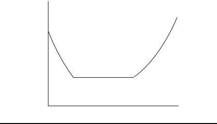
In practice, the hazard function may increase, decrease, remain constant, or indicate a more complicated process. The hazard function for deaths in humans has, for example, the “bathtub” shape shown in Display 12.3. It is relatively high immediately after birth, declines rapidly in the early years, and remains approximately constant before beginning to rise again during late middle age.

h (t)

Display 12.3

12.2.3 Cox’s Regression

Cox’s regression is a semi-parametric approach to survival analysis in which the hazard function is modelled. The method does not require the probability distribution of the survival times to be specified; however, unlike most nonparametric methods, Cox’s regression does use regression parameters in the same way as generalized linear models. The model can be written as:

©2002 CRC Press LLC

where β is a vector of regression parameters and x a vector of covariate values. The hazard functions of any two individuals with covariate vectors xi and xj are assumed to be constant multiples of each other, the multiple being exp[β T(xi – xj)], the hazard ratio or incidence rate ratio. The assumption of a constant hazard ratio is called the proportional hazards assumption. The set of parameters h0(t) is called the baseline hazard function, and can be thought of as nuisance parameters whose purpose is merely to control the parameters of interest β for any changes in the hazard over time. The parameters β are estimated by maximising the partial log-likelihood given by:

where the first summation is over all failures f and the second summation is over all subjects r(f) still alive (and therefore “at risk”) at the time of failure. It can be shown that this log-likelihood is a log profile likelihood (i.e., the log of the likelihood in which the nuisance parameters have been replaced by functions of β which maximise the likelihood for fixed β ). The parameters in a Cox model are interpreted in a similar fashion to those in other regression models met in earlier chapters; that is, the estimated coefficient for an explanatory variable gives the change in the logarithm of the hazard function when the variable changes by one. A more appealing interpretation is achieved by exponentiating the coefficient, giving the effect in terms of the hazard function. An additional aid to interpretation is to calculate

The resulting value gives the percentage change in the hazard function with each unit change in the explanatory variable.

The baseline hazards can be estimated by maximising the full loglikelihood with the regression parameters evaluated at their estimated values. These hazards are nonzero only when a failure occurs. Integrating the hazard function gives the cumulative hazard function

©2002 CRC Press LLC

where H0(t) is the integral of h0(t). The survival curve can be obtained from H(t) using Eq. (12.7).

It follows from Eq. (12.7) that the survival curve for a Cox model is given by:

The log of the cumulative hazard function predicted by the Cox model is given by:

so that the log cumulative hazard functions of any two subjects i and j are parallel with constant difference given by ββ T(xi – xj ).

If the subjects fall into different groups and we are not sure whether we can make the assumption that the group’s hazard functions are proportional to each other, we can estimate separate log cumulative hazard functions for the groups using a stratified Cox model. These curves can then be plotted to assess whether they are sufficiently parallel. For a stratified Cox model, the partial likelihood has the same for m as in Eq. (12.11) except that the risk set for a failure is not confined to subjects in the same stratum.

Survival analysis is described in more detail in Collett (1994) and in Clayton and Hills (1993).

12.3Analysis Using SAS

12.3.1 Gastric Cancer

The data shown in Display 12.1 consist of 89 survival times. There are six values per line except the last line, which has five. The first three values belong to patients in the first treatment group and the remainder to those in the second group. The following data step constructs a suitable SAS data set.

data cancer;

infile 'n:\handbook2\datasets\time.dat' expandtabs missover; do i = 1 to 6;

input temp $ @; censor=(index(temp,'*')>0);

©2002 CRC Press LLC

temp=substr(temp,1,4); days=input(temp,4.); group=i>3;

if days>0 then output; end;

drop temp i; run;

The infilestatement gives the full path name of the file containing the ASCII data. The values are tab separated, so the expandtabs option is used. The missover option prevents SAS from going to a new line if the input statement contains more variables than there are data values, as is the case for the last line. In this case, the variable for which there is no corresponding data is set to missing.

Reading and processing the data takes place within an iterative do loop. The input statement reads one value into a character variable, temp. A character variable is used to allow for processing of the asterisks that indicate censored values, as there is no space between the number and the asterisk. The trailing @ holds the line for further data to be read from it.

If temp contains an asterisk, the index function gives its position; if not, the result is zero. The censor variable is set accordingly. The substr function takes the first four characters of temp and the input function reads this into a numeric variable, days.

If the value of days is greater than zero, an observation is output to the data set. This has the effect of excluding the missing value generated because the last line only contains five values.

Finally, the character variable temp and the loop index variable i are dropped from the data set, as they are no longer needed.

With a complex data step like this, it would be wise to check the resulting data set, for example, with proc print.

Proc lifetest can be used to estimate and compare the survival functions of the two groups of patients as follows:

proc lifetest data=cancer plots=(s); time days*censor(1);

strata group; symbol1 l=1; symbol2 l=3; run;

The plots=(s) option on the proc statement specifies that survival curves be plotted. Log survival (ls), log-log survival (lls), hazard (h), and PDF

©2002 CRC Press LLC

(p) are other functions that may be plotted as well as a plot of censored values by strata (c). A list of plots can be specified; for example, plots=(s,ls,lls).

The time statement specifies the survival time variable followed by an asterisk and the censoring variable, with the value(s) indicating a censored observation in parentheses. The censoring variable must be numeric, with non-missing values for both censored and uncensored observations.

The strata statement indicates the variable, or variables, that determine the strata levels.

Two symbol statements are used to specify different line types for the two groups. (The default is to use different colours, which is not very useful in black and white!)

The output is shown in Display 12.4 and the plot in Display 12.5. In Display 12.4, we find that the median survival time in group 1 is 254 with 95% confidence interval of (193, 484). In group 2, the corresponding values are 506 and (383, 676). The log-rank test for a difference in the survival curves of the two groups has an associated P-value of 0.4521. This suggests that there is no difference in the survival experience of the two groups. The likelihood ratio test (see Lawless [1982]) leads to the same conclusion, but the Wilcoxon test (see Kalbfleisch and Prentice [1980]) has an associated P-value of 0.0378, indicating that there is a difference in the survival time distributions of the two groups. The reason for the difference is that the log-rank test (and the likelihood ratio test) are most useful when the population survival curves of the two groups do not cross, indicating that the hazard functions of the two groups are proportional (see Section 12.2.3). Here the sample survival curves do cross (see Display 12.5) suggesting perhaps that the population curves might also cross. When there is a crossing of the survival curves, the Wilcoxon test is more powerful than the other tests.

©2002 CRC Press LLC

NOTE: The marked survival times are censored observations.

©2002 CRC Press LLC