References

1.J. P. Bentley, Principles of Measurement Systems, 2nd ed., United Kingdom: Longman Scientific and Technical, 1988.

2.E. O. Doebelin, Measurement Systems: Application and Design, 4th ed., New York: McGraw-Hill, 1990.

3.J. P. Holman, Experimental Methods for Engineers, 5th ed., New York: McGraw-Hill, 1989.

4.W. J. Tompkins and J. G. Webster, Interfacing Sensors to the IBM PC, Englewood Cliffs, NJ: PrenticeHall, 1988.

Appendix to Section 6.2

LIST OF MANUFACTURERS

© 1999 by CRC Press LLC

6.3 Capacitive Sensors—Displacement

Halit Eren and Wei Ling Kong

Capacitive sensors are extensively used in industrial and scientific applications. They are based on changes in capacitance in response to physical variations. These sensors find many diverse applications — from humidity and moisture measurements to displacement sensing. In some cases, the basic operational and sensing principles are common in dissimilar applications; and in other cases, different principles can be used for the same applications. For example, capacitive microphones are based on variations of spacing between plates in response to acoustical pressure, thus turning audio signals to variations in capacitance. On the other hand, a capacitive level indicator makes use of the changes in the relative permittivity between the plates. However, capacitive sensors are best known to be associated with displacement measurements for rotational or translational motions, as will be described next. Other applications of capacitance sensors such as humidity and moisture will be discussed.

Capacitive Displacement Sensors

The measurement of distances or displacements is an important aspect of many industrial, scientific, and engineering systems. The displacement is basically the vector representing a change in position of a body or point with respect to a reference point. Capacitive displacement sensors satisfy the requirements of applications where high linearity and wide ranges (from a few centimeters to a couple of nanometers) are needed.

The basic sensing element of a typical displacement sensor consists of two simple electrodes with capacitance C. The capacitance is a function of the distance d (cm) between the electrodes of a structure, the surface area A (cm2) of the electrodes, and the permittivity ε (8.85 × 10–12 F m–1 for air) of the dielectric between the electrodes; therefore:

There are three basic methods for realizing a capacitive displacement sensor: by varying d, A, or ε, as discussed below.

Variable Distance Displacement Sensors

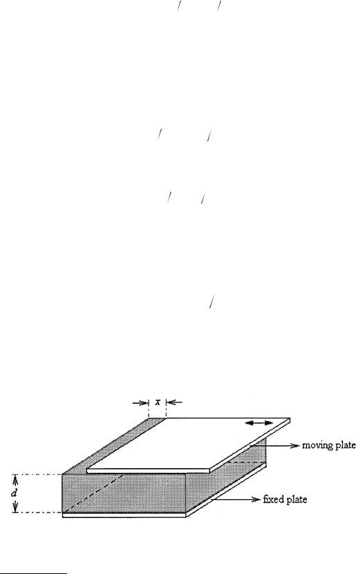
A capacitor displacement sensor, made from two flat coplanar plates with a variable distance x apart, is illustrated in Figure 6.23. Ignoring fringe effects, the capacitance of this arrangement can be expressed by:

FIGURE 6.23 A variable distance capacitive displacement sensor. One of the plates of the capacitor moves to vary the distance between plates in response to changes in a physical variable. The outputs of these transducers are nonlinear with respect to distance x having a hyperbolic transfer function characteristic. Appropriate signal processing must be employed for linearization.

© 1999 by CRC Press LLC

The capacitance of this transducer is nonlinear with respect to distance x, having a hyperbolic transfer function characteristic. The sensitivity of capacitance to changes in plate separation is

Equation 6.24 indicates that the sensitivity increases as x decreases. Nevertheless, from Equations 6.23 and 6.24, it follows that the percent change in C is proportional to the percent change in x. This can be expressed as:

This type of sensor is often used for measuring small incremental displacements without making contact with the object.

Variable Area Displacement Sensors

Alternatively, the displacements may be sensed by varying the surface area of the electrodes of a flat plate capacitor, as illustrated in Figure 6.24. In this case, the capacitance would be:

where w = the width

wx = the reduction in the area due to movement of the plate

Then, the transducer output is linear with displacement x. This type of sensor is normally implemented as a rotating capacitor for measuring angular displacement. The rotating capacitor structures are also used as an output transducer for measuring electric voltages as capacitive voltmeters.

FIGURE 6.24 A variable area capacitive displacement sensor. The sensor operates on the variation in the effective area between plates of a flat-plate capacitor. The transducer output is linear with respect to displacement x. This type of sensor is normally implemented as a rotating capacitor for measuring angular displacement.

© 1999 by CRC Press LLC

FIGURE 6.25 A variable dielectric capacitive displacement sensor. The dielectric material between the two parallel plate capacitors moves, varying the effective dielectric constant. The output of the sensor is linear.

Variable Dielectric Displacement Sensors

In some cases, the displacement may be sensed by the relative movement of the dielectric material between the plates, as shown in Figure 6.25. The corresponding equations would be:

where ε1 = the relative permittivity of the dielectric material

ε2 = the permittivity of the displacing material (e.g., liquid)

In this case, the output of the transducer is also linear. This type of transducer is predominantly used in the form of two concentric cylinders for measuring the level of fluids in tanks. A nonconducting fluid forms the dielectric material. Further discussion will be included in the level measurements section.

Differential Capacitive Sensors

Some of the nonlinearity in capacitive sensors can be eliminated using differential capacitive arrangements. These sensors are basically three-terminal capacitors, as shown in Figure 6.26. Slight variations in the construction of these sensors find many different applications, including differential pressure measurements. In some versions, the central plate moves in response to physical variables with respect to the fixed plates. In others, the central plate is fixed and outer plates are allowed to move. The output from the center plate is zero at the central position and increases as it moves left or right. The range is equal to twice the separation d. For a displacement d, one obtains:

© 1999 by CRC Press LLC

FIGURE 6.26 A differential capacitive sensor. They are essentially three terminal capacitors with one fixed center plate and two outer plates. The response to physical variables is linear. In some versions, the central plate moves in response to physical variable with respect to two outer plates, and in the others, the central plate is fixed and outer plates are allowed to move.

This indicates that the response of the device is more linear than the response of the two plate types. However, in practice some nonlinearity is still observed due to defects in the structure. Therefore, the outputs of these type of sensors still need to be processed carefully, as explained in the signal processing section.

In some differential capacitive sensors, the two spherical depressions are ground into glass disks; then, these are gold-plated to form the fixed plates of a differential capacitor. A thin, stainless-steel diaphragm is clamped between the disks and serves as a movable plate. With equal pressure applied to both ports, the diaphragm is then in neutral position and the output is balanced at a corresponding bridge. If one pressure is greater than the other, the diaphragm deflects proportionally, giving an output due to the differential pressure. For the opposite pressure difference, there is a phase change of 180°. A directionsensitive dc output can be obtained by conventional phase-sensitive demodulation and appropriate filtering. Details of signal processing are given at the end of this chapter. In general, the differential capacitors exhibit better linearity than single-capacitor types.

Integrated Circuit Smart Capacitive Position Sensors

Figure 6.27 shows a typical microstructure capacitive displacement sensor. The sensor consists of two electrodes with capacitance, Cx. Since the system is simple, the determination of the capacitance between the two electrodes is straightforward. The smaller electrode is surrounded by a guard electrode to make Cx independent of lateral and rotational movements of the system parallel to the electrode surface. However, the use of a guard electrode introduces relative deviations in the capacitance Cx between the two electrodes. This is partially true if the size of the guard electrode is smaller than:

© 1999 by CRC Press LLC

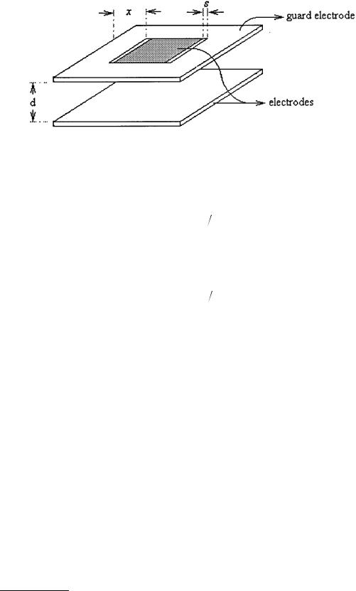
FIGURE 6.27 A typical smart capacitive position sensor. This type of microstructure position sensor contains three electrodes, two of which are fixed and the third electrode moves infinitesimally relative to the others. Although the response is highly nonlinear the integrated chip contains linearization circuits. They feature a 0 mm to 1 mm measuring range with 1 m accuracy.

where x is the width of the guard and d is the distance between the electrodes. Since this deviation introduces nonlinearity, δ is required to be less than 100 ppm. Another form of deviation also exists between the small electrode and the surrounding guard, particularly for gaps

where s is the width of the gap. When the gap width, s, is less than 1/3 of the distance between electrodes, this deviation is negligible.

For signal processing, the system uses the three-signal concept. The capacitor Cx is connected to an inverting operational amplifier and oscillator. If the external movements are linear, by taking into account the parasitic capacitors and offsetting effects, the following equation can be written:

where m is the unknown gain and Moff is the unknown offset. By performing the measurement of a

reference Cref, by measuring the offset, Moff, and by making m = 0, the parameters m and Moff can be eliminated. The final measurement result for the position, Pos, can be defined as:

In this case, the sensor capacitance Cx can be simplified to:

© 1999 by CRC Press LLC

where Ax is the area of the electrode, d0 is the initial distance between them, ε is the dielectric constant, and d is the displacement to be measured. For the reference electrodes, the reference capacitance may be found by:

with Aref the area and dref the distance. Substitution of Equations 6.35 and 6.36 into Equations 6.33 and 6.34 yields:

Pos is a value representing the position if the stable constants a1 and a0 are unknown. The constant a1 = Aref /Ax becomes a stable constant so long as there is good mechanical matching between the electrode

areas. The constant a0 = (Aref d0)/(Ax dref ) is also a stable constant for fixed d0 and dref. These constants are usually determined by calibration repeated over a certain time span. In many applications, these

calibrations are omitted if the displacement sensor is part of a larger system where an overall calibration is necessary. This overall calibration usually eliminates the requirement for a separate determination of

a1 and a0.

The accuracy of this type of system could be as small as 1 µm over a 1 mm range. The total measuring time is better than 0.1 s. The capacitance range is from 1 pF to 50 fF. Interested readers should refer to [4] at the end of this chapter.

Capacitive Pressure Sensors

A commonly used two-plate capacitive pressure sensor is made from one fixed metal plate and one flexible diaphragm, as shown in Figure 6.28. The flat circular diaphragm is clamped around its circumference and bent into a curve by an applied pressure P. The vertical displacement y of this system at any radius r is given by:

FIGURE 6.28 A capacitive pressure sensor. These pressure sensors are made from a fixed metal plate and a flexible diaphragm. The flat flexible diaphragm is clamped around its circumference. The bending of the flexible plate is proportional to the applied pressure P. The deformation of the diaphragm results in changes in capacitance.

© 1999 by CRC Press LLC

where a = the radius of diaphragm

t = the thickness of diaphragm E = Young’s modulus

v = Poisson’s ratio

Deformation of the diaphragm means that the average separation of the plates is reduced. Hence, the

where d is the initial separation of the plates and C is the capacitance at zero pressure.

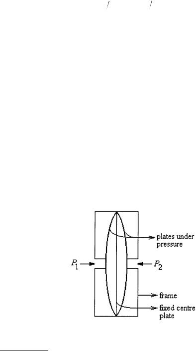
Another type of sensor is the differential capacitance pressure sensor shown in Figure 6.29. The capacitances C1 and C2 of the sensor change with respect to the fixed central plate in response to the applied pressures P1 and P2. Hence, the output of the sensor is proportional to (P1 – P2). The signals are processed using one of the techniques described in the “Signal Processing” section of this chapter.

Capacitive Accelerometers and Force Transducers

In recent years, capacitive-type micromachined accelerometers, as illustrated in Figure 6.30, are gaining popularity. These accelerometers use the proof mass as one plate of the capacitor and use the other plate as the base. When the sensor is accelerated, the proof mass tends to move; thus, the voltage across the capacitor changes. This change in voltage corresponds to the applied acceleration.

In Figure 6.30, let F(x) be the positive force in the direction in which x increases. Neglecting all losses (due to friction, resistance, etc.), the energy balance of the system can be written for an infinitesimally small displacement dx, electrical energy dEe, and field energy dEf of the electrical field between the electrodes as:

FIGURE 6.29 A differential capacitive pressure sensor. The capacitances C1 and C2 of the sensor changes due to deformation in the outer plates, with respect to the fixed central plate in response to the applied pressures P1 and P2.

© 1999 by CRC Press LLC

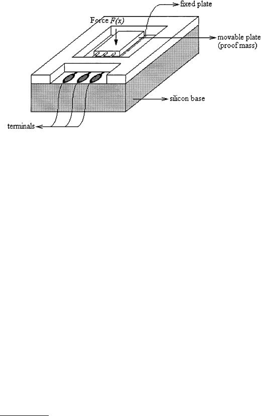
FIGURE 6.30 A capacitive force transducer. A typical capacitive micromachined accelerometer has one of the plates as the proof mass. The other plate is fixed, thus forming the base. When the sensor is accelerated, the proof mass tends to move, thus varying the distance between the plates and altering the voltage across the capacitor. This change in voltage is made to be directly proportional to the applied acceleration.

Also,

If the supply voltage V across the capacitor is kept constant, it follows that dV = 0. Since Q = VC(x), the Coulomb force is given by:

Thus, if the movable electrode has complete freedom of motion, it will have assumed a position in which the capacitance is maximal; also, if C is a linear function of x, the force F(x) becomes independent of x.

Capacitive silicon accelerometers are available in a wide range of specifications. A typical lightweight sensor will have a frequency range of 0 to 1000 Hz, and a dynamic range of acceleration of ±2 g to ±500 g.

Capacitive Liquid Level Measurement

The level of a nonconducting liquid can be determined by capacitive techniques. The method is generally based on the difference between the dielectric constant of the liquid and that of the gas or air above it. Two concentric metal cylinders are used for capacitance, as shown in Figure 6.31. The height of the liquid, h, is measured relative to the total height, l. Appropriate provision is made to ensure that the space between the cylindrical electrodes is filled by the liquid to the same height as the rest of the container. The usual operational conditions dictate that the spacing between the electrodes, s = r2 – r1, should be much less than the radius of the inner electrode, r1. Furthermore, the tank height should be much greater than r2. When these conditions apply, the capacitance is approximated by:

© 1999 by CRC Press LLC

FIGURE 6.31 A capacitive liquid level sensor. Two concentric metal cylinders are used as electrodes of a capacitor. The value of the capacitance depends on the permittivity of the liquid and that of the gas or air above it. The total permittivity changes depending on the liquid level. These devices are usually applied in nonconducting liquid applications.

where εl and εg are the dielectric constants of the liquid and gas (or air), respectively. The denominator of the above equation contains only terms that relate to the fixed system. Therefore, they become a single constant. A typical application is the measurement of the amount of gasoline in a tank in airplanes. The dielectric constant for most compounds commonly found in gasoline is approximately equal to 2, while that of air is approximately unity. A linear change in capacitance with gasoline level is expected for this situation. Quite high accuracy can be achieved if the denominator is kept quite small, thus accentuating the level differences. These sensors often incorporate an ac deflection bridge.

Capacitive Humidity and Moisture Sensors

The permittivities of atmospheric air, of some gases, and of many solid materials are functions of moisture content and temperature. Capacitive humidity devices are based on the changes in the permittivity of the dielectric material between plates of capacitors. The main disadvantage of this type sensor is that a relatively small change in humidity results in a capacitance large enough for a sensitive detection.

Capacitive humidity sensors enjoy wide dynamic ranges, from 0.1 ppm to saturation points. They can function in saturated environments for long periods of time, a characteristic that would adversely affect many other humidity sensors. Their ability to function accurately and reliably extends over a wide range of temperatures and pressures. Capacitive humidity sensors also exhibit low hysteresis and high stability with minimal maintenance requirements. These features make capacitive humidity sensors viable for many specific operating conditions and ideally suitable for a system where uncertainty of unaccounted conditions exists during operations.

© 1999 by CRC Press LLC